分析谐波失真
此示例说明如何分析在具有噪声的情况下弱非线性系统的谐波失真。
简介
在此示例中,我们将研究放大器的简化模型的输出,该放大器的噪声耦合到输入信号并且呈现非线性。我们将研究输入端的衰减如何降低谐波失真。我们还将举例说明如何对放大器输出端的失真在数学上进行校正。
查看非线性的影响
查看放大器非线性影响的一种方便方法是查看用正弦波激励时其输出的周期图。正弦波的振幅设置为放大器的最大允许电压。(2 Vpk)
在此示例中,我们将提供持续时间为 50 毫秒的 2 kHz 正弦波。
VmaxPk = 2;       % Maximum operating voltage
Fi = 2000;        % Sinusoidal frequency of 2 kHz
Fs = 44.1e3;      % Sample rate of 44.1kHz
Tstop = 50e-3;    % Duration of sinusoid
t = 0:1/Fs:Tstop; % Input time vector

% Use the maximum allowable voltage of the amplifier
inputVmax = VmaxPk*sin(2*pi*Fi*t);
outputVmax = helperHarmonicDistortionAmplifier(inputVmax);
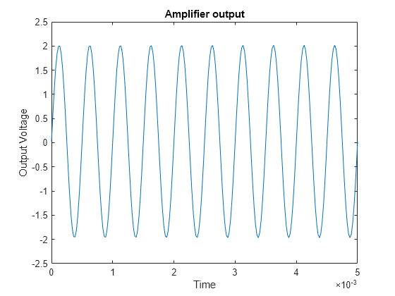
查看输出正弦波的放大区域。请注意,在绘制对时间的图时,很难从视觉上看出放大器的不完美之处。
plot(t, outputVmax)
xlabel("Time (seconds)")
ylabel("Output Voltage (volts)")
axis([0 5e-3 -2.5 2.5])
title("Amplifier output")
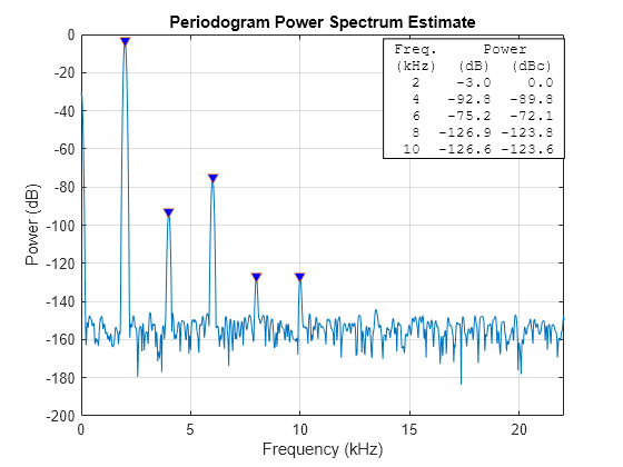
现在我们来查看放大器输出的周期图。
helperPlotPeriodogram(outputVmax, Fs, "power","annotate");

请注意,我们不仅看到输入端的 2 kHz 正弦波,还看到 4 kHz、6 kHz、8 kHz 和 10 kHz 的其他正弦波。这些正弦波是 2 kHz 基频的倍数,这是由于放大器的非线性造成的。
我们还看到相对平坦的噪声功率带。
量化非线性失真
为了便于比较,让我们参考一些常见的失真度量
周期图显示一些定义良好的基波信号的谐波。该图建议我们测量输入信号的总谐波失真,它返回所有谐波成分的功率与基波信号的比率。
thd(outputVmax,Fs)
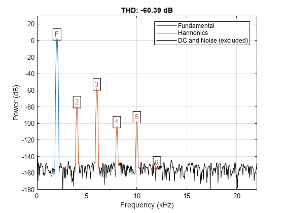
ans =
-60.3888
请注意,第三个(也是最大的)谐波比基波低约 60 dB。大部分失真发生在此处。
我们还可以获得输入中总噪声的估计值。为此,我们调用 SNR,它返回基波功率与所有非谐波成分功率的比率。
snr(outputVmax,Fs)

ans =
130.9300
另一个有用的计算度量是 SINAD。它计算功率与信号中所有其他谐波成分和噪声含量的比率。
sinad(outputVmax, Fs)

ans =
60.3888
THD、SNR 和 SINAD 分别为 -60 dB、131 dB 和 60 dB。由于 THD 的幅值与 SINAD 大致相等,我们可以推断大部分失真是由谐波失真引起的。
如果我们检查周期图,会注意到第三个谐波是输出失真的主要原因。
降低谐波失真的输入衰减
大多数执行放大的模拟电路在谐波失真和噪声功率之间存在固有的折衷。在我们的示例中,与谐波失真相比,我们的放大器具有相对较低的噪声功率。这使得它适合检测低功率信号。如果我们的输入可以衰减到此低功率区域,我们可以恢复一些谐波失真。
让我们通过将输入电压降低二分之一来重复测量。
inputVhalf = (VmaxPk/2) * sin(2*pi*Fi*t);
outputVhalf = helperHarmonicDistortionAmplifier(inputVhalf);
helperPlotPeriodogram(outputVhalf,Fs,"power","annotate");
我们再次使用原先的度量,这次测量降低输入电压后的效果。
thdVhalf = thd(outputVhalf,Fs)
thdVhalf =
-72.0676
snrVhalf = snr(outputVhalf,Fs)
snrVhalf =
124.8767
sinadVhalf = sinad(outputVhalf,Fs)
sinadVhalf =
72.0676
请注意,简单地将输入功率水平衰减 6 dB 会降低谐波成分。SINAD 和 THD 从约 60 dB 提高到了约 72 dB。其代价是 SNR 从 131 dB 降低到了 125 dB。
SNR THD 和 SINAD 当作输入衰减的函数
进一步衰减能否改善整体失真表现?让我们将 THD、SNR 和 SINAD 绘制为输入衰减的函数,从而扫描从 1 dB 到 30 dB 的输入衰减器。
% Allocate a table with 30 entries
nReadings = 30;
distortionTable = zeros(nReadings, 3);

% Compute the THD, SNR and SINAD for each of the attenuation settings
for i = 1:nReadings
  inputVbestAtt = db2mag(-i) * VmaxPk * sin(2*pi*Fi*t);
  outputVbestAtt = helperHarmonicDistortionAmplifier(inputVbestAtt);
  distortionTable(i,:) = [abs(thd(outputVbestAtt,Fs))
                          snr(outputVbestAtt,Fs)
                          sinad(outputVbestAtt,Fs)];
end

% Plot results
plot(distortionTable)
xlabel("Input Attenuation (dB)")
ylabel("Dynamic Range (dB)")
legend("|THD|","SNR","SINAD",Location="best")
title("Distortion Metrics vs. Input Attenuation")

该图显示对应于每个度量的可用动态范围。THD 的幅值对应于无谐波的范围。同样,SNR 对应于不受噪声影响的动态范围;SINAD 对应于没有失真的总动态范围。
从图中可以看出,SNR 随着输入功率衰减的增加而降低。这是因为当您衰减信号时,只有信号在衰减,但放大器的本底噪声保持不变。
还要注意,总谐波失真的幅值会稳步改善,直到它与 SNR 曲线相交,之后测量变得不稳定。当谐波在放大器的噪声下“消失”时,就会出现这种情况。
放大器衰减的一个可行选择项是 26 dB(产生 103 dB 的 SINAD)。这是谐波和噪声失真之间的合理折衷。
% Search the table for the largest SINAD reading
[maxSINAD, iAtten] = max(distortionTable(:,3));
fprintf("Max SINAD (%.1f dB) occurs at %.f dB attenuation\n", ...
  maxSINAD, iAtten)
Max SINAD (103.7 dB) occurs at 26 dB attenuation
让我们绘制衰减器设置为 26 dB 时的周期图。
inputVbestAtt = db2mag(-iAtten) * VmaxPk * sin(2*pi*Fi*t);
outputVbestAtt = helperHarmonicDistortionAmplifier(inputVbestAtt);
helperPlotPeriodogram(outputVbestAtt, Fs, ...
    "power","annotate","shownoise");
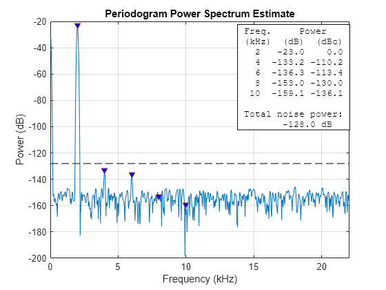
我们还在此处绘制了分布在整个频谱中的总噪声功率水平。请注意,在此衰减设置下,第二个和第三个谐波在频谱中仍然可见,但也远小于总噪声功率。如果我们的应用使用可用频谱的较小带宽,我们将从进一步增加衰减以降低谐波成分中受益。
用于消除失真的后处理
有时我们可以对放大器的一些非线性进行校正。如果放大器的输出经过数字化,我们可以通过对捕获的输出进行数字后处理并对非线性进行数学校正来恢复更有用的动态范围。
在我们的示例中,我们用线性斜坡激励输入,并拟合最适合输入的三次多项式。
inputRamp = -2:0.00001:2;
outputRamp = helperHarmonicDistortionAmplifier(inputRamp);
polyCoeff = polyfit(outputRamp,inputRamp,3)
polyCoeff = 1×4

    0.0010   -0.0002    1.0000   -0.0250
现在我们已经有系数,我们可以在输出端执行后校正,并与原始的未校正输出进行比较。
correctedOutputVmax = polyval(polyCoeff, outputVmax);

helperPlotPeriodogram([outputVmax; correctedOutputVmax],Fs,"power");
subplot(2,1,1)
title("Uncorrected")
subplot(2,1,2)
title("Polynomial Corrected")

请注意,使用多项式校正时,第二个和第三个谐波会显著降低。
让我们用校正后的输出再次重复测量。
thdCorrectedVmax = thd(correctedOutputVmax, Fs)
thdCorrectedVmax =
-99.6194
snrCorrectedVmax = snr(correctedOutputVmax, Fs)
snrCorrectedVmax =
130.7491
sinadCorrectedVmax = sinad(correctedOutputVmax, Fs)
sinadCorrectedVmax =
99.6162
请注意,我们的 SINAD(和 THD)从 60 dB 下降到 99 dB,同时保持 131 dB 的原始 SNR。
组合方法
我们可以将衰减与多项式计算相结合,找到最大限度地降低系统整体 SINAD 的理想工作电压。
subplot(1,1,1)
% Add three more columns to our distortion table
distortionTable = [distortionTable zeros(nReadings,3)];
for i = 1:nReadings
  inputVreduced = db2mag(-i) * VmaxPk * sin(2*pi*Fi*t);
  outputVreduced = helperHarmonicDistortionAmplifier(inputVreduced);
  correctedOutput = polyval(polyCoeff, outputVreduced);
  distortionTable(i,4:6) = [abs(thd(correctedOutput, Fs))
                            snr(correctedOutput, Fs)
                            sinad(correctedOutput, Fs)];
end

h = plot(distortionTable)
h =
  6×1 Line array:

  Line
  Line
  Line
  Line
  Line
  Line
xlabel("Input attenuation (dB)")
ylabel("Dynamic Range (dB)")
for i = 1:3
  h(i+3).Color = h(i).Color;
  h(i+3).LineStyle = "--" ;
end
legend(["|THD|" "SNR" "SINAD"]'+ ...
    [" (uncorrected)" " (corrected)"],Location="best")
title(["Distortion Metrics ..." ...
    "vs. Input Attenuation and Polynomial Correction"]);

在此处,我们对未校正的以及经过多项式校正的放大器的所有三个度量进行了绘图。
从图中可以看出,THD 有显著的改进,而 SNR 不受多项式校正的影响。这在意料之中,因为多项式校正只影响谐波失真,而不影响噪声失真。
让我们显示多项式校正时可能的最大 SINAD
[maxSINADcorrected, iAttenCorr] = max(distortionTable(:,6));
fprintf("Corrected: Max SINAD (%.1f dB) at %.f dB attenuation\n", ...
  maxSINADcorrected, iAttenCorr)
Corrected: Max SINAD (109.7 dB) at 17 dB attenuation
对于经过多项式校正的放大器,放大器衰减的一个良好选择项是 20 dB(产生 109.8 dB 的 SINAD)。使用多项式在最大 SINAD 衰减设置下重新计算放大器。
inputVreduced = db2mag(-iAttenCorr) * VmaxPk * sin(2*pi*Fi*t);
outputVreduced = helperHarmonicDistortionAmplifier(inputVreduced);
correctedOutputVbestAtten = polyval(polyCoeff, outputVreduced);

helperPlotPeriodogram(correctedOutputVbestAtten, Fs, ...
    "power","annotate","shownoise");
title("Periodogram of attenuated and polynomial corrected amplifier")
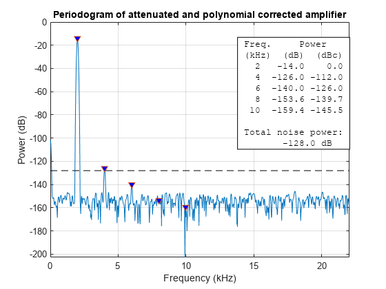
请注意,在理想衰减设置下,通过多项式校正,除了第二个谐波以外的所有谐波都应完全消失。如前所述,第二个谐波出现在总噪声基底功率水平的正下方。这在使用放大器全部带宽的应用中提供了合理的折衷。
总结
我们演示了如何对出现失真的放大器输出应用多项式校正,以及如何选择合理的衰减值来降低谐波失真的影响。