thd

This example shows explicitly how to calculate the total harmonic distortion in dBc for a signal consisting of the fundamental and two harmonics. The explicit calculation is checked against the result returned by thd.

Create a signal sampled at 1 kHz. The signal consists of a 100 Hz fundamental with amplitude 2 and two harmonics at 200 and 300 Hz with amplitudes 0.01 and 0.005. Obtain the total harmonic distortion explicitly and using thd.

t = 0:0.001:1-0.001;
x = 2*cos(2*pi*100*t)+0.01*cos(2*pi*200*t)+0.005*cos(2*pi*300*t);
tharmdist = 10*log10((0.01^2+0.005^2)/2^2)

tharmdist = 
-45.0515

r = thd(x)

r = 
-45.0515

Create a signal sampled at 1 kHz. The signal consists of a 100 Hz fundamental with amplitude 2 and three harmonics at 200, 300, and 400 Hz with amplitudes 0.01, 0.005, and 0.0025.

Set the number of harmonics to 3. This includes the fundamental. Accordingly, the power at 100, 200, and 300 Hz is used in the THD calculation.

t = 0:0.001:1-0.001;
x = 2*cos(2*pi*100*t)+0.01*cos(2*pi*200*t)+ ...
    0.005*cos(2*pi*300*t)+0.0025*sin(2*pi*400*t);
r = thd(x,1000,3)

r = 
-45.0515

Specifying the number of harmonics equal to 3 ignores the power at 400 Hz in the THD calculation.

Create a signal sampled at 1 kHz. The signal consists of a 100 Hz fundamental with amplitude 2 and three harmonics at 200, 300, and 400 Hz with amplitudes 0.01, 0.005, and 0.0025, respectively.

t = 0:0.001:1-0.001;
fs = 1000;
x = 2*cos(2*pi*100*t) + 0.01*cos(2*pi*200*t)+ ...
    0.005*cos(2*pi*300*t) + 0.0025*sin(2*pi*400*t);

Obtain the periodogram PSD estimate of the signal and use the PSD estimate as the input to compute the THD. Set the number of harmonics to 3. This includes the fundamental frequency component. Accordingly, the powers at 100, 200, and 300 Hz are used in the THD calculation.

[pxx,f] = periodogram(x,rectwin(length(x)),length(x),fs);
r = thd(pxx,f,3,"psd")

r = 
-45.0515

Determine the THD by inputting the power spectrum obtained with a Hamming window and the resolution bandwidth of the window.

Create a signal sampled at 10 kHz. The signal consists of a 100 Hz fundamental with amplitude 2 and three odd-numbered harmonics at 300, 500, and 700 Hz with amplitudes 0.01, 0.005, and 0.0025, respectively.

fs = 10000;
t = 0:1/fs:1-1/fs;
x = 2*cos(2*pi*100*t) + 0.01*cos(2*pi*300*t)+ ...
    0.005*cos(2*pi*500*t) + 0.0025*sin(2*pi*700*t);

Compute the THD from the power spectrum of the signal. Specify the number of harmonics to 7.

sigLength = length(x);
win = hamming(sigLength);
[sxx,f] = periodogram(x,win,sigLength,fs,"power");
rbw = enbw(win,fs);

r = thd(sxx,f,rbw,7,"power")

r = 
-44.8396

Generate a signal that resembles the output of a weakly nonlinear amplifier with a 2.1 kHz tone as input. The signal is sampled for 1 second at 10 kHz. Compute and plot the power spectrum of the signal. Use a Kaiser window with β = 38 for the computation.

Fs = 10000;
f = 2100;

t = 0:1/Fs:1; 
x = tanh(sin(2*pi*f*t)+0.1) + 0.001*randn(1,length(t));

periodogram(x,kaiser(length(x),38),[],Fs,'power')

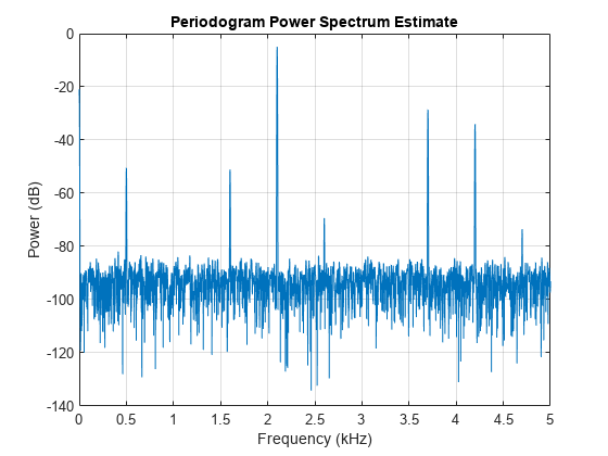
Harmonics stick out from the noise at frequencies of 4.2 kHz, 6.3 kHz, 8.4 kHz, 10.5 kHz, 12.6 kHz, and 14.7 kHz. All frequencies except for the first one are greater than the Nyquist frequency. The harmonics are aliased respectively into 3.7 kHz, 1.6 kHz, 0.5 kHz, 2.6 kHz, and 4.7 kHz.

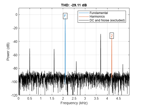
Compute the total harmonic distortion of the signal. By default, thd treats the aliased harmonics as part of the noise.

thd(x,Fs,7);

Repeat the computation, but now treat the aliased harmonics as part of the signal.

thd(x,Fs,7,'aliased');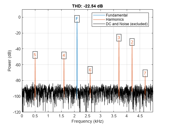

Create a signal sampled at 10 kHz. The signal consists of a 100 Hz fundamental with amplitude 2 and three odd-numbered harmonics at 300, 500, and 700 Hz with amplitudes 0.01, 0.005, and 0.0025. Specify the number of harmonics to 7. Determine the THD, the power at the harmonics, and the corresponding frequencies.

fs = 10000;
t = 0:1/fs:1-1/fs;
x = 2*cos(2*pi*100*t)+0.01*cos(2*pi*300*t)+ ...
    0.005*cos(2*pi*500*t)+0.0025*sin(2*pi*700*t);
[r,harmpow,harmfreq] = thd(x,10000,7);
[harmfreq harmpow]

ans = 7×2

  100.0000    3.0103
  201.0000 -321.0983
  300.0000  -43.0103
  399.0000 -281.9259
  500.0000  -49.0309
  599.0000 -282.1066
  700.0000  -55.0515

The powers at the even-numbered harmonics are on the order of $$-300$$ dB, which corresponds to an amplitude of $$10^{-15}$$.

Generate a sinusoid of frequency 2.5 kHz sampled at 50 kHz. Add Gaussian white noise with standard deviation 0.00005 to the signal. Pass the result through a weakly nonlinear amplifier. Plot the THD.

fs = 5e4;
f0 = 2.5e3;
N = 1024;
t = (0:N-1)/fs;

ct = cos(2*pi*f0*t);
cd = ct + 0.00005*randn(size(ct));

amp = [1e-5 5e-6 -1e-3 6e-5 1 25e-3];
sgn = polyval(amp,cd);
thd(sgn,fs);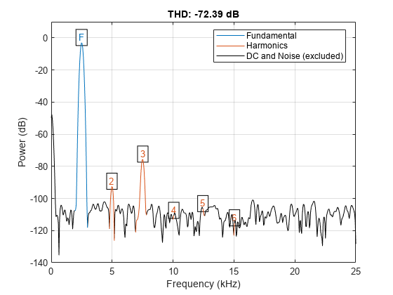

The plot shows the spectrum used to compute the ratio and the region treated as noise. The DC level is excluded from the computation. The fundamental and harmonics are labeled.