Main Content

toi

Third-order intercept point

Description

oip3 = toi(x) returns the output third-order intercept (TOI) point, in decibels (dB), of a real sinusoidal two-tone input signal, x. The computation is performed over a periodogram of the same length as the input using a Kaiser window with β = 38.

oip3 = toi(x,fs) specifies the sample rate, fs. The default value of fs is 1.

example

oip3 = toi(pxx,f,'psd') specifies the input as a one-sided power spectral density (PSD), pxx, of a real signal. f is a vector of frequencies that corresponds to the vector of pxx estimates.

example

oip3 = toi(sxx,f,rbw,'power') specifies the input as a one-sided power spectrum, sxx, of a real signal. rbw is the resolution bandwidth over which each power estimate is integrated.

example

[oip3,fundpow,fundfreq,imodpow,imodfreq] = toi(___) also returns the power, fundpow, and frequencies, fundfreq, of the two fundamental sinusoids. It also returns the power, imodpow, and frequencies, imodfreq, of the lower and upper intermodulation products. This syntax can use any of the input arguments in the preceding syntaxes.

example

toi(___) with no output arguments plots the spectrum of the signal and annotates the lower and upper fundamentals (f1, f2) and intermodulation products (2f1 – f2, 2f2 – f1). Higher harmonics and intermodulation products are not labeled. The TOI appears above the plot.

example

Examples

collapse all

Create a two-tone sinusoid with frequencies f1=5 kHz and f2=6 kHz, sampled at 48 kHz. Make the signal nonlinear by feeding it to a polynomial. Add noise. Set the random number generator to the default settings for reproducible results. Compute the third-order intercept point. Verify that the intermodulation products occur at 2f2-f1=4 kHz and 2f1-f2=7 kHz.

rng default
fi1 = 5e3;
fi2 = 6e3;
Fs = 48e3;
N = 1000;
x = sin(2*pi*fi1/Fs*(1:N))+sin(2*pi*fi2/Fs*(1:N));
y = polyval([0.5e-3 1e-7 0.1 3e-3],x)+1e-5*randn(1,N);

[myTOI,Pfund,Ffund,Pim3,Fim3] = toi(y,Fs);
myTOI,Fim3
myTOI = 
1.3844
Fim3 = 1×2
103 ×

    4.0002    6.9998

Create a two-tone sinusoid with frequencies 5 kHz and 6 kHz, sampled at 48 kHz. Make the signal nonlinear by evaluating a polynomial. Add noise. Set the random number generator to the default settings for reproducible results.

rng default
fi1 = 5e3;
fi2 = 6e3;
Fs = 48e3;
N = 1000;
x = sin(2*pi*fi1/Fs*(1:N))+sin(2*pi*fi2/Fs*(1:N));
y = polyval([0.5e-3 1e-7 0.1 3e-3],x)+1e-5*randn(1,N);

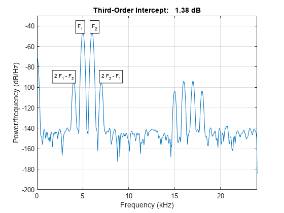
Evaluate the periodogram of the signal using a Kaiser window. Compute the TOI using the power spectral density. Plot the result.

w = kaiser(numel(y),38);

[Sxx, F] = periodogram(y,w,N,Fs,'psd');
[myTOI,Pfund,Ffund,Pim3,Fim3] = toi(Sxx,F,'psd')
myTOI = 
1.3843
Pfund = 1×2

  -22.9133  -22.9132

Ffund = 1×2
103 ×

    5.0000    6.0000

Pim3 = 1×2

  -71.4868  -71.5299

Fim3 = 1×2
103 ×

    4.0002    6.9998

toi(Sxx,F,'psd');

Figure contains an axes object. The axes object with title Third-Order Intercept: 1.38 dB, xlabel Frequency (kHz), ylabel Power/frequency (dB/Hz) contains 5 objects of type line, text.

Create a two-tone sinusoid with frequencies 5 kHz and 6 kHz, sampled at 48 kHz. Make the signal nonlinear by evaluating a polynomial. Add noise. Set the random number generator to the default settings for reproducible results.

rng default

fi1 = 5e3;
fi2 = 6e3;
Fs = 48e3;
N = 1000;

x = sin(2*pi*fi1/Fs*(1:N))+sin(2*pi*fi2/Fs*(1:N));
y = polyval([0.5e-3 1e-7 0.1 3e-3],x)+1e-5*randn(1,N);

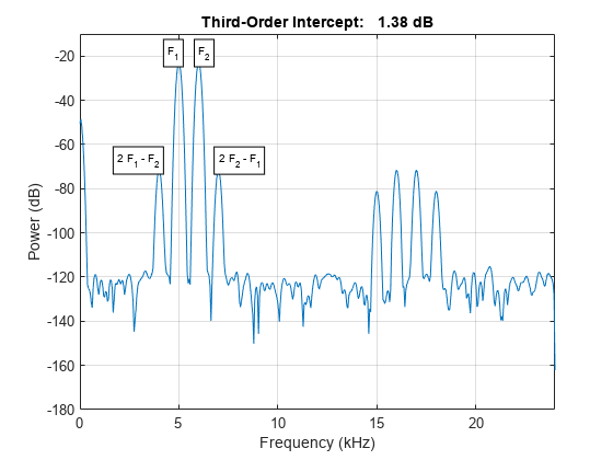
Evaluate the periodogram of the signal using a Kaiser window. Compute the TOI using the power spectrum. Plot the result.

w = kaiser(numel(y),38);

[Sxx,F] = periodogram(y,w,N,Fs,'power');

toi(Sxx,F,enbw(w,Fs),'power')

Figure contains an axes object. The axes object with title Third-Order Intercept: 1.38 dB, xlabel Frequency (kHz), ylabel Power (dB) contains 5 objects of type line, text.

ans = 
1.3844

Generate 640 samples of a two-tone sinusoid with frequencies 5 Hz and 7 Hz, sampled at 32 Hz. Make the signal nonlinear by evaluating a polynomial. Add noise with standard deviation 0.01. Set the random number generator to the default settings for reproducible results. Compute the third-order intercept point. Verify that the intermodulation products occur at 2f2-f1=9Hz and 2f1-f2=3Hz.

rng default
x = sin(2*pi*5/32*(1:640))+cos(2*pi*7/32*(1:640));
q = x + 0.01*x.^3 + 1e-2*randn(size(x));
[myTOI,Pfund,Ffund,Pim3,Fim3] = toi(q,32)
myTOI = 
17.4230
Pfund = 1×2

   -2.8350   -2.8201

Ffund = 1×2

    5.0000    7.0001

Pim3 = 1×2

  -43.1362  -43.5211

Fim3 = 1×2

    3.0015    8.9744

Generate 640 samples of a two-tone sinusoid with frequencies 5 Hz and 7 Hz, sampled at 32 Hz. Make the signal nonlinear by evaluating a polynomial. Add noise with standard deviation 0.01. Set the random number generator to the default settings. Plot the spectrum of the signal. Display the fundamentals and the intermodulation products. Verify that the latter occur at 9 Hz and 3 Hz.

rng default
x = sin(2*pi*5/32*(1:640))+cos(2*pi*7/32*(1:640));
q = x + 0.01*x.^3 + 1e-2*randn(size(x));
toi(q,32)

Figure contains an axes object. The axes object with title Third-Order Intercept: 17.42 dB, xlabel Frequency (Hz), ylabel Power (dB) contains 5 objects of type line, text.

ans = 
17.4230

Input Arguments

collapse all

Real-valued sinusoidal two-tone signal, specified as a row or column vector.

Example: polyval([0.01 0 1 0],sum(sin(2*pi*[5 7]'*(1:640)/32))) + 0.01*randn([1 640])

Data Types: double | single

Sample rate, specified as a positive real scalar. The sample rate is the number of samples per unit time. If the unit of time is seconds, then the sample rate has units of hertz.

Data Types: double | single

One-sided power spectral density estimate, specified as a real-valued, nonnegative row or column vector.

The power spectral density must be expressed in linear units, not decibels. Use db2pow to convert decibel values to power values.

Example: [pxx,f] = periodogram(cos(pi./[4;2]*(0:159))'+randn(160,2)) specifies the periodogram PSD estimate of a noisy two-channel sinusoid sampled at 2π Hz and the frequencies at which it is computed.

Data Types: double | single

Cyclical frequencies corresponding to the one-sided PSD estimate, pxx, specified as a row or column vector. The first element of f must be 0.

Data Types: double | single

Power spectrum, specified as a real-valued nonnegative row or column vector.

The power spectrum must be expressed in linear units, not decibels. Use db2pow to convert decibel values to power values.

Example: [sxx,w] = periodogram(cos(pi./[4;2]*(0:159))'+randn(160,2),'power') specifies the periodogram power spectrum estimate of a two-channel sinusoid embedded in white Gaussian noise and the normalized frequencies at which it is computed.

Data Types: double | single

Resolution bandwidth, specified as a positive scalar. The resolution bandwidth is the product of the frequency resolution of the discrete Fourier transform and the equivalent noise bandwidth of the window.

Data Types: double | single

Output Arguments

collapse all

Output third-order intercept point of a sinusoidal two-tone signal, returned as a real-valued scalar expressed in decibels. If the second primary tone is the second harmonic of the first primary tone, then the lower intermodulation product is at zero frequency. The function returns NaN in those cases.

Data Types: double | single

Power contained in the two fundamental sinusoids of the input signal, returned as a real-valued two-element row vector.

Data Types: double | single

Frequencies of the two fundamental sinusoids of the input signal, returned as a real-valued two-element row vector.

Data Types: double | single

Power contained in the lower and upper intermodulation products of the input signal, returned as a real-valued two-element row vector.

Data Types: double | single

Frequencies of the lower and upper intermodulation products of the input signal, returned as a real-valued two-element row vector.

Data Types: double | single

References

[1] Kundert, Kenneth S. "Accurate and Rapid Measurement of IP2 and IP3." Designer's Guide Community. May, 2002. https://designers-guide.org/analysis/intercept-point.pdf.

Extended Capabilities

Version History

Introduced in R2013b
See Also

| | |