AR Order Selection with Partial Autocorrelation Sequence

Open Live Script

This example shows how to assess the order of an autoregressive model using the partial autocorrelation sequence. For a stationary time series with values $X (1), X (2), X (3), \dots, X (k + 1)$ , the partial autocorrelation sequence at lag $k$ is the correlation between $X (1)$ and $X (k + 1)$ after regressing $X (1)$ and $X (k + 1)$ on the intervening observations, $X (2), X (3), X (4), \dots, X (k)$ . For a moving average process, you can use the autocorrelation sequence to assess the order. However, for an autoregressive (AR) or autoregressive moving average (ARMA) process, the autocorrelation sequence does not help in order selection. This example uses the following workflow for model order selection in an AR process:

Simulates a realization of the AR(2) process.
Graphically explores the correlation between lagged values of the time series.
Examines the sample autocorrelation sequence of the time series.
Fits an AR(15) model to the time series by solving the Yule-Walker equations (aryule).
Uses the reflection coefficients returned by aryule to compute the partial autocorrelation sequence.
Examines the partial autocorrelation sequence to select the model order.

Consider the AR(2) process defined by

$X (n) + 1.5 X (n - 1) + 0.75 X (n - 2) = ε (n),$

where $ε (n)$ is an $N (0, 1)$ Gaussian white noise process. Simulate a 1000-sample time series from the AR(2) process defined by the difference equation. Set the random number generator to the default settings for reproducible results.

A = [1 1.5 0.75];
rng default
x = filter(1,A,randn(1000,1));

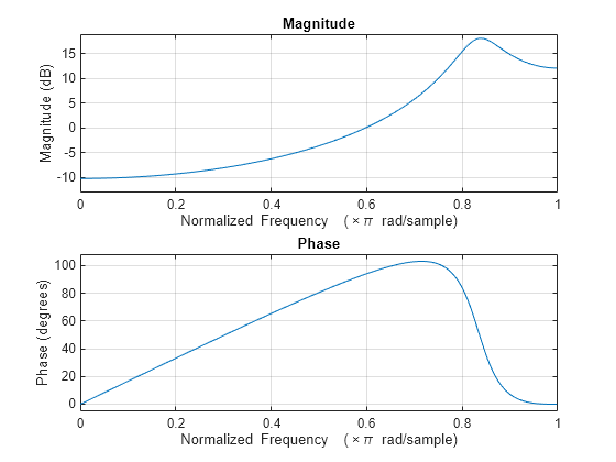
View the frequency response of the AR(2) process.

freqz(1,A)

$Figure contains 2 axes objects. Axes object 1 with title Phase, xlabel Normalized Frequency (\times\pi rad/sample), ylabel Phase (degrees) contains an object of type line. Axes object 2 with title Magnitude, xlabel Normalized Frequency (\times\pi rad/sample), ylabel Magnitude (dB) contains an object of type line.$

The AR(2) process acts like a highpass filter in this case.

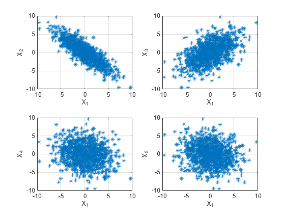
Graphically examine the correlation in x by producing scatter plots of $X (n + 1)$ vs. $X (1)$ for $n = 2, 3, 4, 5$ .

figure
for k = 1:4
    subplot(2,2,k)
    plot(x(1:end-k),x(k+1:end),'*')
    xlabel('X_1')
    ylabel(['X_' int2str(k+1)])
    grid
end

In the scatter plot, you see a linear relationship between $X (1)$ and $X (2)$ and between $X (1)$ and $X (3)$ , but not between $X (1)$ and either $X (4)$ or $X (5)$ .

The points in the top row scatter plots fall approximately on a line with a negative slope in the top left panel and positive slope in the top right panel. The scatter plots in the bottom two panels do not show any apparent linear relationship.

The negative correlation between $X (1)$ and $X (2)$ and the positive correlation between $X (1)$ and $X (3)$ are explained by the highpass-filter behavior of the AR(2) process.

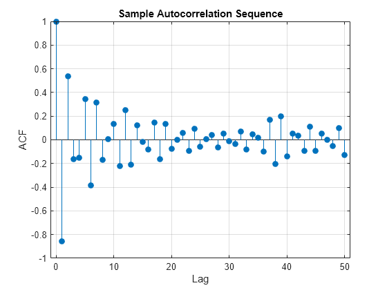
Find the sample autocorrelation sequence up to lag 50 and plot the result.

[xc,lags] = xcorr(x,50,'coeff');

figure
stem(lags(51:end),xc(51:end),'filled')
xlabel('Lag')
ylabel('ACF')
title('Sample Autocorrelation Sequence')
grid

Figure contains an axes object. The axes object with title Sample Autocorrelation Sequence, xlabel Lag, ylabel ACF contains an object of type stem.

The sample autocorrelation sequence shows a negative value at lag 1 and a positive value at lag 2. Based on the scatter plot, this result is expected. However, you cannot determine the appropriate order for the AR model from the sample autocorrelation sequence.

Fit an AR(15) model using aryule. Return the sequence of reflection coefficients, whose negative is the partial autocorrelation sequence.

[arcoefs,E,K] = aryule(x,15);
pacf = -K;

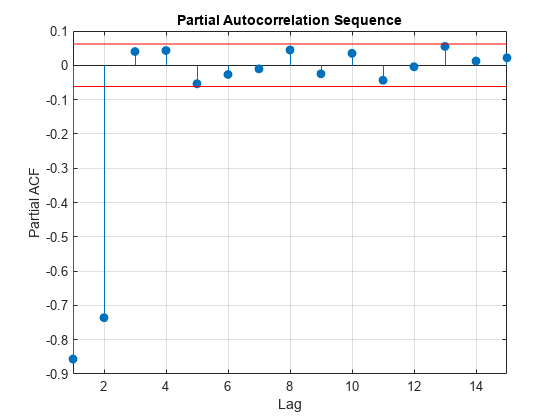
Plot the partial autocorrelation sequence along with the large-sample 95% confidence intervals. If the data are generated by an autoregressive process of order $p$ , the values of the sample partial autocorrelation sequence for lags greater than $p$ follow a $N (0, 1 / N)$ distribution, where $N$ is the length of the time series. For a 95% confidence interval, the critical value is $\sqrt{2} {e r f}^{- 1} (0.95) \approx 1.96$ and the confidence interval is $Δ = 0 \pm 1.96 / \sqrt{N}$ .

stem(pacf,'filled')
xlabel('Lag')
ylabel('Partial ACF')
title('Partial Autocorrelation Sequence')
xlim([1 15])

conf = sqrt(2)*erfinv(0.95)/sqrt(1000);
hold on
plot(xlim,[1 1]'*[-conf conf],'r')
hold off
grid

Figure contains an axes object. The axes object with title Partial Autocorrelation Sequence, xlabel Lag, ylabel Partial ACF contains 3 objects of type stem, line.

The only values of the partial autocorrelation sequence outside the 95% confidence bounds occur at lags 1 and 2. This indicates that the correct model order for the AR process is 2.

In this example, you generated the time series to simulate an AR(2) process. The partial autocorrelation sequence only confirms that result. In practice, you have only the observed time series without any prior information about model order. In a realistic scenario, the partial autocorrelation sequence is an important tool for appropriate model order selection in stationary autoregressive time series.

AR Order Selection with Partial Autocorrelation Sequence

See Also