Measure Power of Deterministic Periodic Signals

Signal Classification

In general, signals can be classified into three broad categories, power signals, energy signals, or neither. Deterministic signals which are made up of sinusoids, are an example of power signals, which have infinite energy but finite average power. Random signals also have finite average power and fall into the category of power signals. A transient signal is an example of energy signals, which start and end with zero amplitude. There are still other signals that cannot be characterized as either power signals or energy signals.

Theoretical Power of a Single Sinusoid

As a first example, estimate the average power of a sinusoidal signal with a peak amplitude of 1 and a frequency component at 128 Hz.

Fs = 1024;
t = 0:1/Fs:1-(1/Fs);
A = 1;
F1 = 128;
x = A*sin(2*pi*t*F1);

Plot a portion of the signal in the time domain.

idx = 1:128;
plot(t(idx),x(idx))
ylabel('Amplitude')
xlabel('Time (seconds)')
axis tight
grid

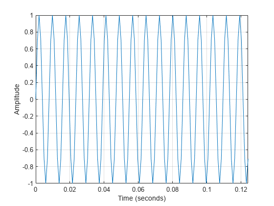
The theoretical average power (mean-square) of each complex sinusoid is ${\mathit{A}}^2/4$, which in this example is 0.25 or –6.02 dB. So, accounting for the power in the positive and negative frequencies results in an average power of $2\times {\mathit{A}}^2/4$.

power_theoretical = (A^2/4)*2

power_theoretical = 
0.5000

Compute in dB the power contained in the positive frequencies:

pow2db(power_theoretical/2)

ans = 
-6.0206

Measuring the Power of a Single Sinusoid

To measure the average power of the signal, call periodogram and specify the 'power' option.

periodogram(x,hamming(length(x)),[],Fs,'centered','power')
ylim([-10 -5.5])

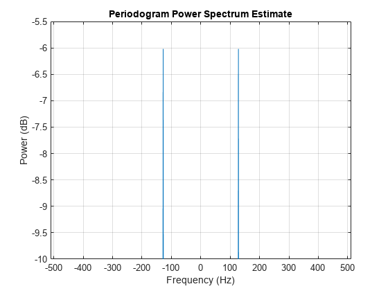
As you can see from the zoomed-in portion of the plot, each complex sinusoid has an average power of roughly –6 dB.

Estimating the Power of a Single Sinusoid via PSD

Another way to calculate the average power of a signal is by "integrating" the area under the PSD curve.

periodogram(x,hamming(length(x)),[],Fs,'centered','psd')

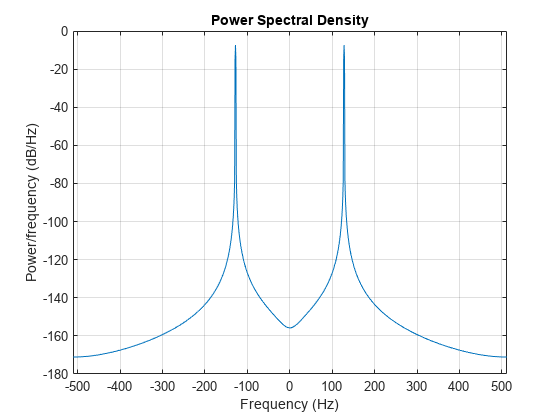
In this plot, the peaks of the spectrum plot do not have the same height as in the power spectrum plot. The heights are different because it is the area under the curve — which is the measure of the average power — that matters when taking power spectral density (PSD) measurements. To verify that statement, use the bandpower function, which calculates the average power using the rectangle approximation to integrate under the curve.

[Pxx_hamming,F] = periodogram(x,hamming(length(x)),[],Fs,'psd');
power_freqdomain = bandpower(Pxx_hamming,F,'psd')

power_freqdomain = 
0.5000

According to Parseval's theorem, the total average power of a sinusoid is the same in both the time domain and the frequency domain. Use that fact to check the value of the signal's estimated total average power by summing up the signal in the time domain.

power_timedomain = sum(abs(x).^2)/length(x)

power_timedomain = 
0.5000

Theoretical Power of Multiple Sinusoids

For the second example, estimate the total average power of a signal containing energy at multiple frequency components: one at DC with amplitude 1.5, one at 100 Hz with amplitude 4, and one at 200 Hz with amplitude 3.

Fs = 1024;
t  = 0:1/Fs:1-(1/Fs);
Ao = 1.5;
A1 = 4;
A2 = 3;
F1 = 100;
F2 = 200;
x  = Ao + A1*sin(2*pi*t*F1) + A2*sin(2*pi*t*F2);

Plot the first 128 samples of the signal.

idx = 1:128;
plot(t(idx),x(idx))
grid
ylabel('Amplitude')
xlabel('Time (seconds)')

As in the previous example, the theoretical average power of each complex sinusoid is ${\mathit{A}}^2/4$. The DC average power of the signal is equal to its peak power (since it is constant) and therefore is given by ${\mathit{A}}_0^2$. Accounting for the power in the positive and negative frequencies results in a total average power value (sum of the average power of each harmonic component) of ${\mathit{A}}_0^2+2\times {\mathit{A}}_1^2/4+2\times {\mathit{A}}_2^2/4$ for the signal.

power_theoretical = Ao^2 + (A1^2/4)*2 + (A2^2/4)*2

power_theoretical = 
14.7500

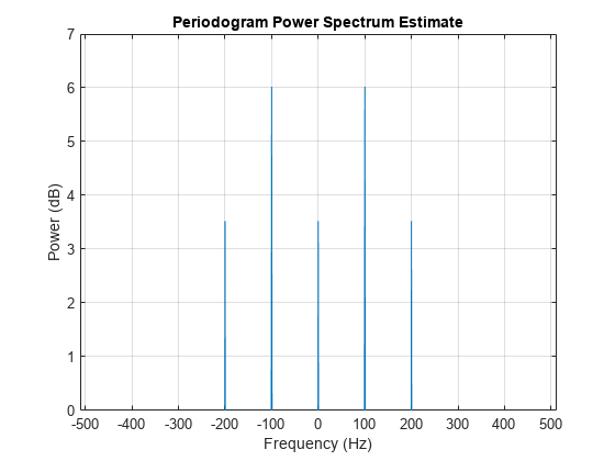
Calculate the average power of each unique frequency component in dB to see that the theoretical results match the mean-square spectrum plot below.

pow2db([Ao^2 A1^2/4 A2^2/4])

ans = 1×3

    3.5218    6.0206    3.5218

Measuring the Power of Multiple Sinusoids

To measure once again the average power of the signal, use the periodogram function once more to calculate and plot the power spectrum of the signal.

periodogram(x,hamming(length(x)),[],Fs,'centered','power')
ylim([0 7])

Estimating the Power of Multiple Sinusoids Using PSD

As in the first example, estimate the total average power of the signal by "integrating" under the PSD curve.

periodogram(x,hamming(length(x)),[],Fs,'centered','psd')

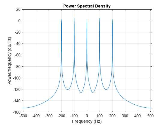
Once again the height of the peaks of the spectral density plot at a specific frequency component may not match the ones of the plot of the power spectrum. The difference is due to the reasons noted in the first example.

[Pxx, F] = periodogram(x, hamming(length(x)),[],Fs,'centered','psd');
power_freqdomain = bandpower(Pxx,F,'psd')

power_freqdomain = 
14.7500

Again verify the estimated average power of the signal by invoking Parseval's theorem and summing up the signal in the time domain.

power_timedomain = sum(abs(x).^2)/length(x)

power_timedomain = 
14.7500

Relationship between Power Spectrum, Power Spectral Density and ENBW

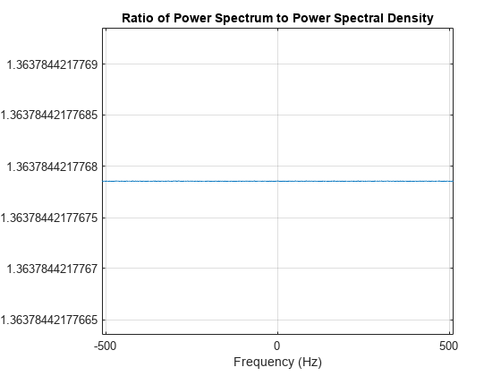
You may have noticed that, while the height of the peaks of the power and power spectral density plots are different, the ratio of one to the other is constant.

Pxx = periodogram(x,hamming(length(x)),[],Fs,'centered','psd');
Sxx = periodogram(x,hamming(length(x)),[],Fs,'centered','power');

plot(F,Sxx./Pxx)
grid
axis tight
xlabel('Frequency (Hz)')
title('Ratio of Power Spectrum to Power Spectral Density')

ratio = mean(Sxx./Pxx)

ratio = 
1.3638

The ratio of power to power spectral density is related to the two-sided equivalent noise bandwidth (ENBW) of the window. You can compute this ratio directly by calling the enbw function with the window and its corresponding sample rate as input arguments.

bw = enbw(hamming(length(x)),Fs)

bw = 
1.3638

Enhanced Power Measurements Using Reassigned Periodogram

In the previous sections, power was measured from one or multiple sinusoids having a frequency that coincided with a bin. Peak power estimates are usually less accurate when the signal frequency is out of bin. To see this effect, create a sinusoid with a non-integer number of cycles over a one-second period.

Fs = 1024;
t = 0:1/Fs:1-(1/Fs);
A = 1;
F = 20.4;
x = A*sin(2*pi*F*t);
nfft = length(x);
power_theoretical = pow2db(A^2/4*2);

Create a Hamming window and a flat top window.

w1 = hamming(length(x));
w2 = flattopwin(length(x));

Compute the periodogram of x using the Hamming window. Zoom in on the peak.

h1 = figure;
stem(F,power_theoretical,'BaseValue',-50);

[Pxx1,f1] = periodogram(x,w1,nfft,Fs,'power');

hold on
plot(f1,pow2db(Pxx1),'+-')

axis([0 40 -45 0])
legend('Theoretical','Periodogram')
xlabel('Frequency (Hz)')
ylabel('Power (dB)')
title('Periodogram Power Spectrum Estimate')
grid

The peak power estimate is below the theoretical peak, and the frequency of the peak estimate differs from the true frequency.

[Pmax,imax] = max(Pxx1);
dPmax_w1 = pow2db(Pmax) - power_theoretical

dPmax_w1 = 
-1.1046

dFreq = f1(imax) - F

dFreq = 
-0.4000

Reduce Amplitude Error with Zero-Padding

To see why this is happening, compute the periodogram using a larger number of FFT bins.

[Pxx2,f2] = periodogram(x,w1,100*nfft,Fs,'power');

figure
stem(F,power_theoretical,'BaseValue',-50)

hold on
plot(f1,pow2db(Pxx1),'+')
plot(f2,pow2db(Pxx2))
hold off

axis([0 40 -40 0])
legend('Theoretical Peak','nfft = 1024','nfft = 102400')
xlabel('Frequency (Hz)')
ylabel('Power (dB)')
title('Periodogram Power Spectrum Estimate')
grid

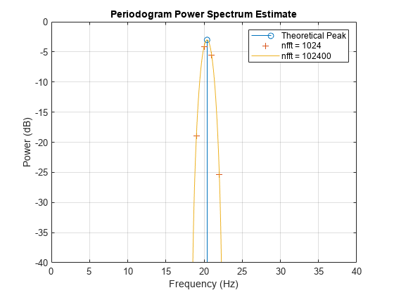
In the original periodogram, the spectral peak is located between two bins, and for that reason the estimated peak is below the theoretical peak. Increasing the number of FFT bins gives a better picture of the spectrum, although this may be a computationally expensive way to improve peak measurements.

Reduce Amplitude Error with a Flat Top Window

Another way to produce a better estimate for the peak amplitude is to use a different window. Compute the periodogram of x using the flat top window.

[Pxx,F1] = periodogram(x,w2,nfft,Fs,'power');

figure(h1)
plot(F1,pow2db(Pxx))
legend('Theoretical','Hamming','Flat Top')
hold off

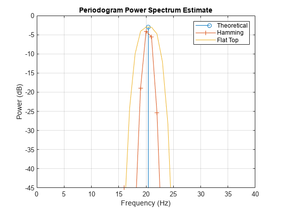
The flat top window is broad and flat. It produces a peak estimate closer to the theoretical value when x does not contain an integer number of cycles, and hence the spectral peak does not fall exactly on a bin.

dPmax_w2 = pow2db(max(Pxx)) - power_theoretical

dPmax_w2 = 
-6.2007e-04

The broader peak that the flat top window produces could be a disadvantage when trying to resolve closely spaced peaks, and the frequency of the measured peak is again different from the frequency of the theoretical peak.

Reduce Amplitude Error with Reassigned Periodogram

Now add the 'reassigned' flag to periodogram. Periodogram reassignment uses phase information, which is normally discarded, to reassign the signal to its center of energy. The procedure can result in sharper spectral estimates. Plot the reassigned periodogram of x and zoom in on the peak. Use the Hamming window and the flat top window.

[RPxx1,~,~,Fc1] = periodogram(x,w1,nfft,Fs,'power','reassigned');
[RPxx2,~,~,Fc2] = periodogram(x,w2,nfft,Fs,'power','reassigned');

stem(F,power_theoretical,'*','BaseValue',-40)
hold on
stem(Fc1,pow2db(RPxx1),'BaseValue',-50)
stem(Fc2,pow2db(RPxx2),'BaseValue',-50)
hold off

legend('Theoretical','Hamming Reassignment','Flattop Reassignment')
xlabel('Frequency (Hz)')
ylabel('Power (dB)')
title('Periodogram Power Spectrum Estimate')
axis([19.5 21 -4 -2])
grid

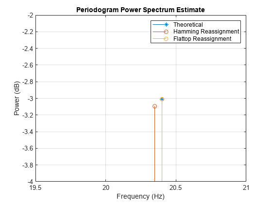
The reassigned estimates of power are closer to the theoretical value for both windows, with the flat top window producing the best peak measurement.

[RPxx1max,imax1] = max(RPxx1);
[RPxx2max,imax2] = max(RPxx2);
dPmax_reassign_w1 = pow2db(RPxx1max) - power_theoretical

dPmax_reassign_w1 = 
-0.0845

dPmax_reassign_w2 = pow2db(RPxx2max) - power_theoretical

dPmax_reassign_w2 = 
-1.1131e-05

The frequency estimates are also improved using the reassigned periodogram, with the flat top window again giving the best results.

Fc1(imax1)-F

ans = 
-0.0512

Fc2(imax2)-F

ans = 
5.6552e-04