Prediction Polynomial

Open Live Script

This example shows how to obtain the prediction polynomial from an autocorrelation sequence. The example also shows that the resulting prediction polynomial has an inverse that produces a stable all-pole filter. You can use the all-pole filter to filter a wide-sense stationary white noise sequence to produce a wide-sense stationary autoregressive process.

Create an autocorrelation sequence defined by

$r (k) = \frac{24}{5} 2^{- | k |} - \frac{27}{10} 3^{- | k |}, k = 0, 1, 2 .$

k = 0:2;
rk = (24/5)*2.^(-k)-(27/10)*3.^(-k);

Use ac2poly to obtain the prediction polynomial of order 2, which is

$A (z) = 1 - \frac{5}{6} z^{- 1} + \frac{1}{6} z^{- 2} .$

A = ac2poly(rk);

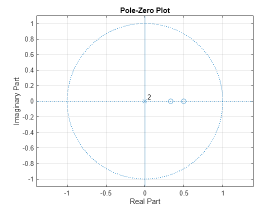
Examine the pole-zero plot of the FIR filter to see that the zeros are inside the unit circle.

zplane(A,1)
grid

Figure contains an axes object. The axes object with title Pole-Zero Plot, xlabel Real Part, ylabel Imaginary Part contains 4 objects of type line, text. One or more of the lines displays its values using only markers

The inverse all-pole filter is stable with poles inside the unit circle.

zplane(1,A)
grid
title('Poles and Zeros')

Figure contains an axes object. The axes object with title Poles and Zeros, xlabel Real Part, ylabel Imaginary Part contains 4 objects of type line, text. One or more of the lines displays its values using only markers

Use the all-pole filter to produce a realization of a wide-sense stationary AR(2) process from a white-noise sequence. Set the random number generator to the default settings for reproducible results.

rng default

x = randn(1000,1);
y = filter(1,A,x);

Compute the sample autocorrelation of the AR(2) realization and show that the sample autocorrelation is close to the true autocorrelation.

[xc,lags] = xcorr(y,2,'biased');
[xc(3:end) rk']

ans = 3×2

    2.2401    2.1000
    1.6419    1.5000
    0.9980    0.9000