Single-Sideband Amplitude Modulation

This example shows how to use the Hilbert transform to carry out single-sideband (SSB) amplitude modulation (AM) of a signal. Single-sideband AM signals have less bandwidth than normal AM signals.

Generate 512 samples of a simulated broadband signal using the sinc function. Specify a bandwidth of $$\pi /4$$ rad/sample.

N = 512;
n = 0:N-1;

bw = 1/4;
x = sinc((n-N/2)*bw);

Add white Gaussian noise such that the signal-to-noise ratio is 20 dB. Reset the random number generator for reproducible results. Use the periodogram function to estimate the power spectral density (PSD) of the signal.

rng default

SNR = 20;
noise = randn(size(x))*std(x)/db2mag(SNR);
x = x + noise;

periodogram(x)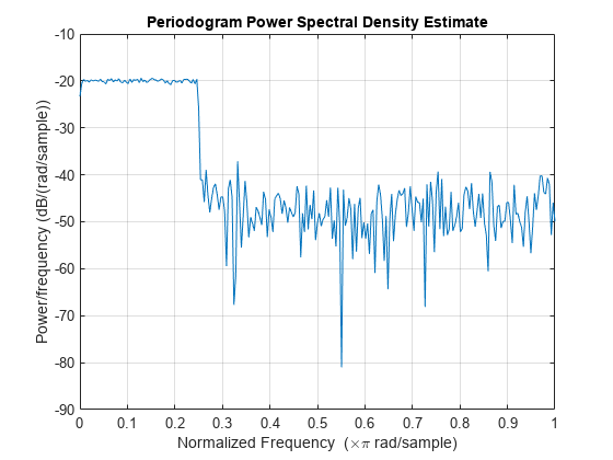

Amplitude modulate the signal using a cosine of carrier frequency $${\omega }_c=\pi /2$$. Multiply by $$\sqrt{2}$$ so that the power of the modulated signal equals the power of the original signal. Estimate the PSD.

wc = pi/2;

x1 = x.*cos(wc*n)*sqrt(2);

periodogram(x1)
legend("Modulated")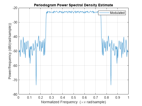

SSB amplitude modulation reduces the bandwidth of the signal by half. To carry out SSB amplitude modulation, you must first compute the Hilbert transform of the signal. Then, amplitude modulate the signal using a sine with the same carrier frequency, $${\omega }_c$$, as before, and add it to the previous signal.

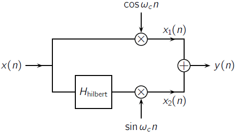
Design a Hilbert transformer using the designfilt function. Specify a filter order of 64 and a transition width of 0.1. Filter the signal.

Hhilbert = designfilt("hilbertfir",FilterOrder=64, ...
    TransitionWidth=0.1);

xh = filter(Hhilbert,x);

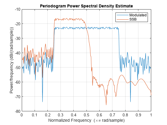
Use the grpdelay function to determine the delay, gd, introduced by the filter. Compensate for the delay by discarding the first gd points of the filtered signal and padding with zeros at the end. Amplitude modulate the result and add it to the original. Compare the PSDs.

gd = mean(grpdelay(Hhilbert));
xh = xh(gd+1:end);
eh = zeros(size(x));
eh(1:length(xh)) = xh;

x2 = eh.*sin(wc*n)*sqrt(2);

y = x1+x2;

periodogram([x1;y]')
legend(["Modulated" "SSB"])

Downconvert the signal and estimate the PSD.

ym = y.*cos(wc*n)*sqrt(2);

periodogram(ym)
legend("Downconverted")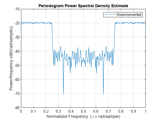

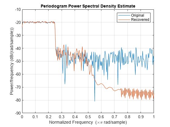
Lowpass filter the modulated signal to recover the original. Specify a 64th-order FIR lowpass filter with a cutoff frequency of $$\pi /2$$. Compensate for the delay introduced by the filter.

d = designfilt('lowpassfir',FilterOrder=64, ...
    CutoffFrequency=0.5);
dem = filter(d,ym);

gd = mean(grpdelay(d));
dem = dem(gd+1:end);

dm = zeros(size(x));
dm(1:length(dem)) = dem;

Estimate the PSD of the filtered signal and compare it to that of the original.

periodogram([x;dm]')
legend(["Original" "Recovered"])

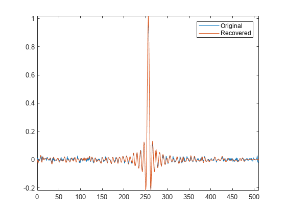
Use the snr function to compare the signal-to-noise ratios of the two signals. Plot the two signals in the time domain.

snrOrig = snr(x,noise)

snrOrig = 
20.0259

snrRecv = snr(dm,noise)

snrRecv = 
20.1373

plot(n,[x;dm]')
legend(["Original" "Recovered"])
axis tight

References

Buck, John R., Michael M. Daniel, and Andrew C. Singer. Computer Explorations in Signals and Systems Using MATLAB. 2nd Edition. Upper Saddle River, NJ: Prentice Hall, 2002.

See Also

designfilt | periodogram | snr