View, Preprocess, and Write EDF File

View EDF File

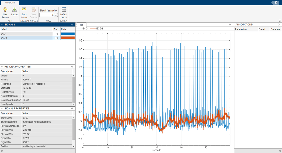
The example.edf file contains two ECG signals that each have six data records. The sample rate is 128 Hz and each data record duration is 10 seconds. Import the file into EDF File Analyzer to view the signals:

Preprocess Data Stored in EDF File

Baseline wander is low-frequency noise caused by a person's breathing or motion. It is common to remove baseline wander before analyzing an ECG signal. You can interactively remove baseline wander by applying a bandpass filter in Signal Analyzer.

Read the ECG data into a timetable. Each row in the timetable is a cell array that corresponds to a data record. To successfully plot and preprocess the timetable data in Signal Analyzer, concatenate the vectors in each column to obtain a single vector for each ECG signal.

tt = edfread("example.edf");
Fs = 128;

sig1 = vertcat(tt.ECG{:});
sig2 = vertcat(tt.ECG2{:});

Open Signal Analyzer and drag both signals to the display. To add time information, select both signals in the Signal table and on the Analyzer tab, select Time Values. Select Sample Rate and Start Time and specify a sample rate of 128 Hz and a start time of 0 s. Click OK.

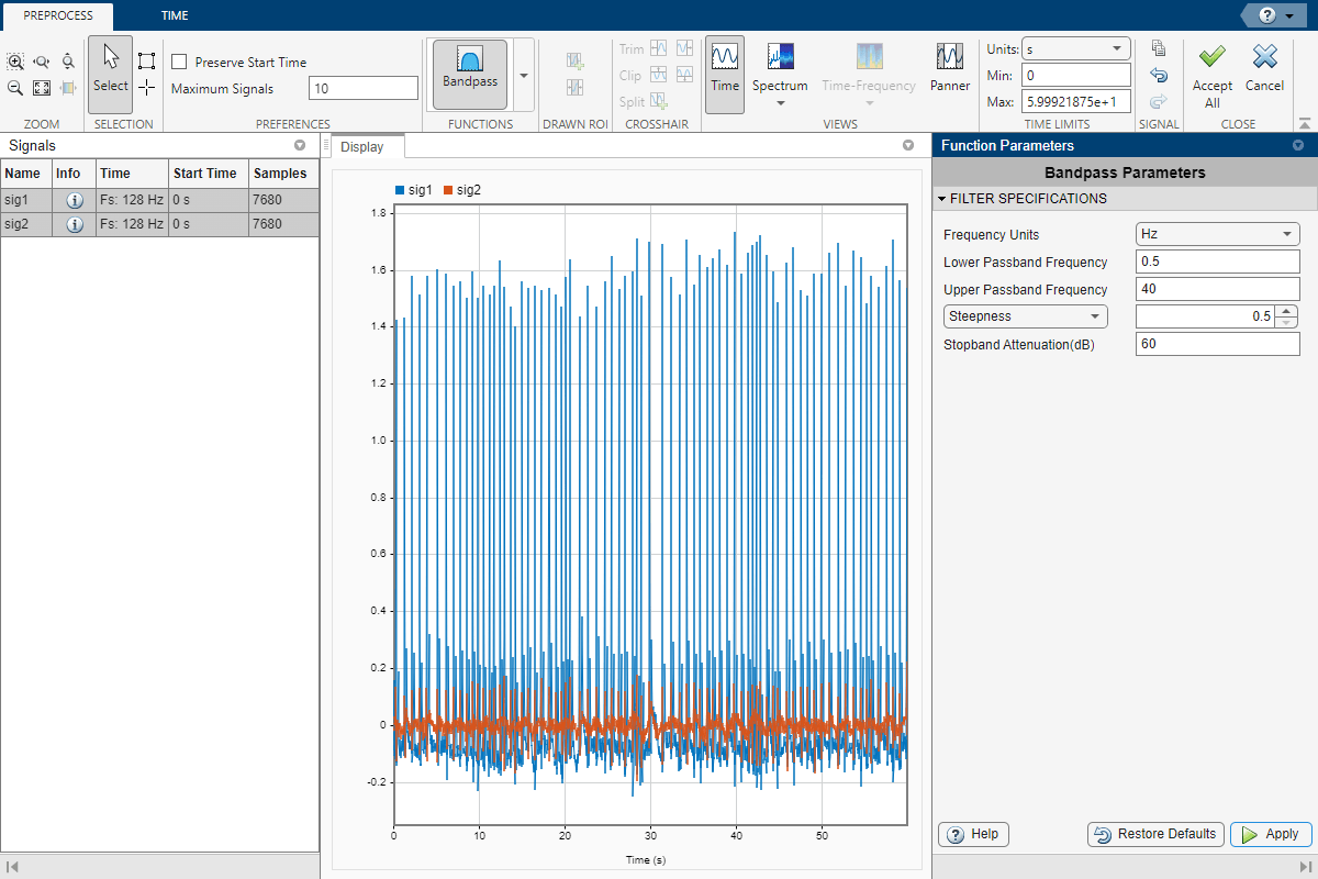
Select sig1 and sig2 in the Signal table. On the Analyzer tab, click Preprocess to enter the preprocessing mode. With both signals selected, select Bandpass from the Functions gallery. In the Function Parameters panel, specify the lower and upper passband frequencies as 0.5 Hz and 40 Hz, respectively. Set the steepness to 0.5. Click Apply to apply the filter to the selected signals.

Click Accept All to save the preprocessing results and exit the mode.

Locate QRS Regions

Rename the signals as sig1_Bandpass and sig2_Bandpass. Either right-click the signal name and select Rename or double-click the signal name. Export the filtered signals to the Workspace.

Use the helperLocateQRS function to locate the QRS intervals of the first signal using a windowing algorithm. The helperLocateQRS function is defined at the end of this example.

load sig1_Bandpass
qrsROIs = helperLocateQRS(sig1_Bandpass,Fs);

Create Annotations for QRS Intervals

Create a timetable of annotations that correspond to the QRS intervals.

Onset = seconds(qrsROIs(:,1)/Fs);
Duration = seconds(diff(qrsROIs,1,2)/Fs);
Annotations = repelem("QRS",size(qrsROIs,1))';

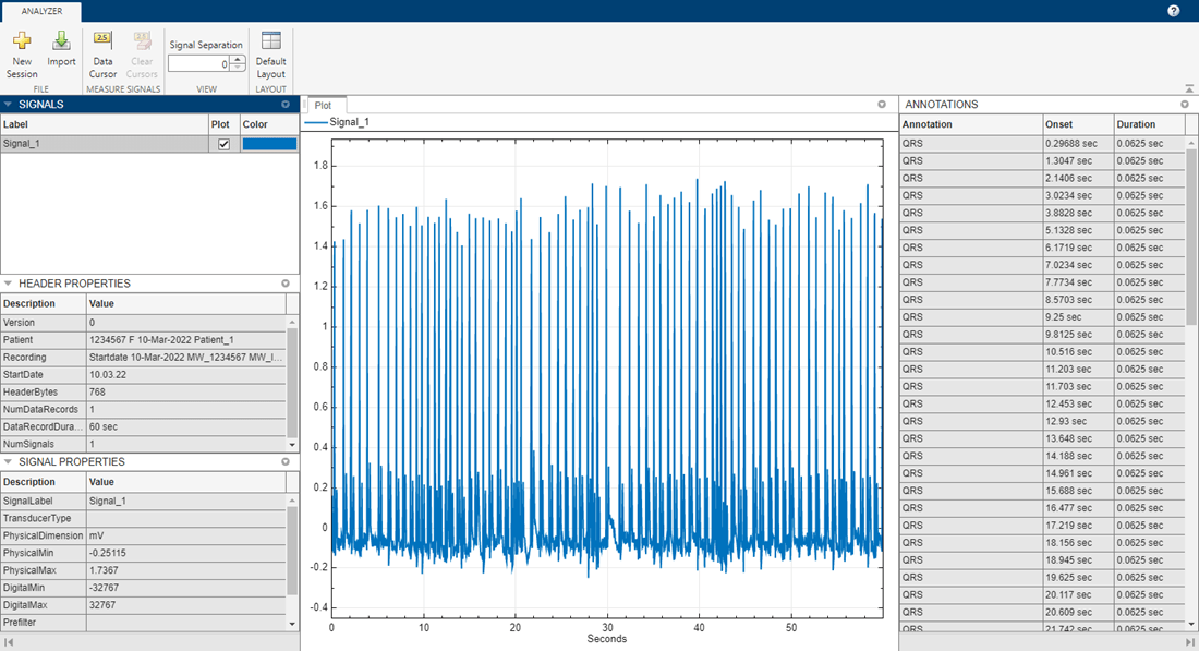
annotationslist = timetable(Onset,Annotations,Duration)

annotationslist=76×2 timetable
       Onset       Annotations     Duration 
    ___________    ___________    __________

    0.29688 sec       "QRS"       0.0625 sec
    1.3047 sec        "QRS"       0.0625 sec
    2.1406 sec        "QRS"       0.0625 sec
    3.0234 sec        "QRS"       0.0625 sec
    3.8828 sec        "QRS"       0.0625 sec
    5.1328 sec        "QRS"       0.0625 sec
    6.1719 sec        "QRS"       0.0625 sec
    7.0234 sec        "QRS"       0.0625 sec
    7.7734 sec        "QRS"       0.0625 sec
    8.5703 sec        "QRS"       0.0625 sec
    9.25 sec          "QRS"       0.0625 sec
    9.8125 sec        "QRS"       0.0625 sec
    10.516 sec        "QRS"       0.0625 sec
    11.203 sec        "QRS"       0.0625 sec
    11.703 sec        "QRS"       0.0625 sec
    12.453 sec        "QRS"       0.0625 sec
      ⋮

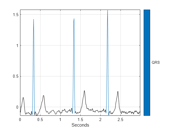
Use a signalMask object and the plotsigroi function to visualize the first three QRS intervals.

msk = signalMask(table(qrsROIs/Fs,Annotations),SampleRate=Fs);
plotsigroi(msk,sig1_Bandpass(1:3*Fs))

Write EDF File

Write a new EDF file that contains sig1_Bandpass and its annotations.

hdr = edfheader("EDF");
hdr.NumDataRecords = 1;
hdr.DataRecordDuration = seconds(length(sig1_Bandpass)/Fs);
hdr.NumSignals = 1;
hdr.PhysicalDimensions = "mV";
hdr.PhysicalMin = min(sig1_Bandpass);
hdr.PhysicalMax = max(sig1_Bandpass);
hdr.DigitalMin = -32767;
hdr.DigitalMax = 32767;
edfw = edfwrite("filteredECG.edf",hdr,sig1_Bandpass,annotationslist,InputSampleType="physical");

Import the new EDF file, filteredECG, into EDF File Analyzer to visualize the filtered signal and QRS annotations.

helperLocateQRS Function

Locate the QRS intervals in an ECG signal using a modified windowing algorithm from [1]. This method first finds the R-peaks of the signal using a minimum threshold equal to 0.4 times the maximum value of the signal. The algorithm then finds the Q-peaks by computing the minimum value of the signal in a window starting 50 ms before the corresponding R-peak and ending at this peak. The algorithm finds the S-peaks by computing the minimum value of the signal in a window starting at the corresponding R-peak and ending 50 ms after this peak. The QRS interval is defined as the time interval from the Q-peak to the S-peak.

function qrsROIs = helperLocateQRS(ECG,Fs)
[~,locs] = findpeaks(ECG,MinPeakHeight=0.4*max(ECG));
for i = 1:length(locs)
    qstart = floor(locs(i)-(Fs*.05));
    qwin = [qstart locs(i)];
    [~,qidx] = min(ECG(qwin));
    qidx = qidx+qstart;
    qloc(i,1) = qidx;
    
    swin = [locs(i) round(locs(i)+(Fs*.055))];
    [~,sidx] = min(ECG(swin));
    sidx = sidx+locs(i);
    sloc(i,1) = sidx;
end
qrsROIs = [qloc sloc];
end

References

[1] Umer, Muhammad, Bilal Ahmed Bhatti, Muhammad Hammad Tariq, Muhammad Zia-ul-Hassan, Muhammad Yaqub Khan, and Tahir Zaidi. “Electrocardiogram Feature Extraction and Pattern Recognition Using a Novel Windowing Algorithm.” Advances in Bioscience and Biotechnology 05, no. 11 (2014): 886–94. https://doi.org/10.4236/abb.2014.511103.