SimBiology.function.SimFunction
Function-like object to simulate SimBiology models
Description
The SimFunction object provides an interface that allows you
to execute a SimBiology® model like a function and a workflow to perform parameter scans (in parallel if
Parallel Computing Toolbox™ is available), Monte Carlo simulations, and scans with multiple or vectorized
doses. Because a SimFunction object can be executed like a function handle,
you can customize it to integrate SimBiology models with other MATLAB® products and other custom analyses (such as visual predictive
checks).
Creation
Use createSimFunction to construct a
SimFunction object. SimFunction objects are immutable once
created and automatically accelerated at the first function execution. After creation, you can
run the SimFunction object (F) using the syntaxes
described next.
Syntax
Description
SimFunction Created With Doses
If you specified dosing information when you called createSimFunction to construct the SimFunction object
F, then F has the following syntaxes.
simdata = F(phi,t_stop,u,t_output)SimData object
simdata after simulating a SimBiology model using the initial
conditions or simulation scenarios specified in phi, simulation
stop time, t_stop, dosing information, u, and
output time, t_output.
SimFunction Created Without Doses
If you did not specify any dosing information when you called
createSimFunction, then F has the following
syntaxes:
simdata = F(phi,t_stop)SimData object
simdata after simulating the model using initial conditions or
simulation scenarios specified in phi, and simulation stop time,
t_stop.
simdata = F(phi,t_stop,[],t_output)phi, t_stop, empty
dosed argument [], and t_output. You must
specify u, the dosing information, as an empty
array[] for this signature. When t_output is
empty and t_stop is specified, the simulations report the solver
time points until t_stop. When t_output is
specified and t_stop is empty, only the time points in
t_output are reported. When both are specified, the reported time
points are the union of solver time points and the time points in
t_output. If the last t_output is greater
than the corresponding t_stop, then simulation proceeds until the
last time point in t_output.
[ returns T,Y] =
F(_)T, a cell array of numeric vector, and
Y, a cell array of 2-D numeric matrices, using any of the input
arguments in the preceding syntaxes.
Input Arguments
Initial conditions or simulation scenarios, specified as one of the following.
Empty array
[]or empty cell array{}, meaning to perform simulations using the baseline initial values, that is, the values listed in theParameterproperty of theSimFunctionobject, without altering them.Matrix of size S-by-P, where S is the number of simulations to perform and P is the number of parameters specified in the
paramsargument when you calledcreateSimFunctionto constructF. Each simulation is performed with the parameters specified in the corresponding row ofphi.S-by-V matrix of variant objects or a cell column vector of length S, where each element consists of a row vector of variant objects. S is the number of simulations to perform, and V is the number of variant objects. These variants are only allowed to modify the
SimFunctioninput parameters, that is, model elements that were specified as theparamsinput argument when you calledcreateSimFunction. In other words, you must specify the variant parameters as the input parameters when you create theSimFunctionobject. AnySimFunctioninput parameters that are not specified in the variants use their baseline initial values.If, within a row of variants, multiple entries refer to the same model element, the last occurrence is used for simulation.
Scalar
SimBiology.Scenariosobject containing S number of scenarios.
When phi is specified as a
1-by-P or
1-by-V matrix (or a Scenarios
object with only one scenario), then all simulations use the same parameters, and the
number of simulations is determined from the t_stop,
u, or t_output argument in that order. For
example, if phi and t_stop have a single row
and u is a matrix of size
N-by-DoseTargets, the number of simulations is
determined as N.
When phi is specified as a
SimBiology.Scenarios object, all scenarios are simulated. Variants
are applied before values from the scenarios are set.
Simulation stop time, specified as a nonnegative scalar or numeric vector.
Specify a nonnegative scalar to use as the same stop time for all simulations.
Specify a numeric vector of size N to use as a stop time for each simulation in a total of N simulations.
Data Types: double
Doses to use during simulation, specified as one of the following.
Empty array
[]to apply no doses during simulation unless you specifyphias aScenariosobject that has doses defined in its entries.tableof dosing information with two or three variables containingScheduleDosedata (ScheduleDosetable), namely, dose time, dose amount, and dose rate (optional). Name the table variables as follows.u.Properties.VariableNames = {'Time','Amount','Rate'};If
UnitConversionis on, specify units for each variable. For instance, you can specify units as follows.u.Properties.VariableUnits = {'second','molecule','molecule/second'};This table can have multiple rows, where each row represents a dose applied to the dose target at a specified dose time with a specified amount and rate if available.
tablewith one row and five variables containingRepeatDosedata (RepeatDosetable). Dose rate variable is optional. Name the variables as follows.u.Properties.VariableNames = {'StartTime','Amount','Rate','Interval','RepeatCount'};If
UnitConversionis on, specify units for each variable. Units for'RepeatCount'variable can be empty''or'dimensionless'. The unit of the'Amount'variable must be dimensionally consistent with that of the target species. For example, if the unit of target species is in an amount unit (such as mole or molecule), then the'Amount'variable unit must have the same dimension, i.e., its unit must be an amount unit and cannot be a mass unit (such as gram or kilogram). The unit for the'Rate'variable must be dimensionally consistent as well.u.Properties.VariableUnits = {'second','molecule','molecule/second','second','dimensionless'};Tip
If you already have a dose object (
ScheduleDoseorRepeatDose), you can get this dose table by using thegetTablemethod of the object.Cell array of tables of size 1-by-N, where N is the number of dose targets. Each cell can represent either table as described previously.
Cell array of tables of size S-by-N, where S is the number of simulations and N is the number of dose targets. Each cell represents a table. S is equal to the number of rows in
phi.If
uis a cell array of tables, then:If
phiis also aScenariosobject, the combined number of doses in theScenariosobject and the number of columns inumust equal to the number of elements in theDosedproperty of theSimFunctionobject. In other words, the dosing information that you specified during the creation of theSimFunctionobject must be consistent with the dosing information you specify in the execution of the object. The total number of elements for theDosedproperty is equal to the combination of any doses from the inputScenariosobject and doses in the dosed input argument ofcreateSimFunction.If
phiis not aScenariosobject, the number of columns (N) in the cell arrayumust be equal to the number of elements in theDosedproperty of theSimFunctionobject. The order of dose tables must also match the order of dosed species increateSimFunction. That is, SimBiology assumes one-to-one correspondence between the columns ofuand dose targets specified in theDosedproperty of theSimFunctionobject, meaning the doses (dose tables) in the first column ofuare applied to the first dose target in theDosedproperty and so on.The ith dose for the jth dose target is ignored if
u{i,j} = [].If the ith dose is not parameterized,
u{i,j}can be[]or either type of table (theScheduleDoseorRepeatDosetable).If the ith dose is parameterized,
u{i,j}must be[]or aRepeatDosetable with one row and a column for each property (StartTime,Amount,Rate,Interval,RepeatCount) that is not parameterized. It is not required to create a column for a dose property that is parameterized. If all of the properties are parameterized, you can pass in a table with one row and no columns to specify the parameterized dose is applied during simulations. To create such table, usetable.empty(1,0).
Data Types: double | table | cell
Output times, specified as one of the following.
Vector of monotonically increasing output times that is applied to all simulations
Cell array containing a single time vector that is applied to all simulations
Cell array of vectors representing output times. The ith cell element provides the output times for the ith simulation. The number of elements in the cell array must match the number of rows (simulations) in
phi.
Data Types: double | cell
Time course data and dosing information, specified as a table or dataset.
tbl contains information such as group labels, independent
variable, dependent variables, dose amounts, and dose rates. You must name the
variables of the table or data set as
'GROUP','TIME','DEPENDENTVAR1','DEPENDENTVAR2',...,'AMOUNT1','RATE1','AMOUNT2','RATE2',....
The rate variable is optional for each dose.
If the Dosed property of the SimFunction
object F is empty, then amount- and rate-related variables are not
required. The number of groups in tbl must be equal to the number
of rows, or the number of scenarios, in phi. The combined dosing
information in phi, if phi is a
SimBiology.Scenarios object, and the number of amount and rate
columns in tbl must be equal to the number of doses in the
Dosed property of the object F. If
tbl has additional columns, they are ignored.
If UnitConversion is on, specify a unit
for each variable. The unit of 'Amount' variable must be
dimensionally consistent with that of the target species. See the description of the
input argument u for details.
Data Types: table
Properties
This property is read-only.
SimFunction input parameters, specified as a table. The table has the following variables.
'Name''Value''Type''Units'(only ifUnitConversionis turned on)
The table contains information about model quantities (species, compartments, or
parameters) that define the inputs of a SimFunction object. For
instance, this table can contain parameters or species whose values are being scanned by
the SimFunction object.
Data Types: table
This property is read-only.
Responses or outputs of SimFunction, specified as a table.
The table has the following variables.
'Name''Type''Units'(only ifUnitConversionis turned on)
This table contains information about model quantities (species, compartments, or
parameters) that are the outputs of a SimFunction object.
Data Types: table
This property is read-only.
Dosing information, specified as a table.
The table has the following variables.
'TargetName''TargetDimension'(only ifUnitConversionis turned on)
In addition, the table also contains variables for each property that is
parameterized. For each parameterized property, two variables are added to this table.
The first variable has the same name as the property name and the value is the name of
the specified parameter. The second variable has the property name suffixed by
Value (PropertyNameValue), and the value is the
default value of the parameter. If the UnitConversion is on, the unit
column is also added with the name PropertyNameUnits.
Suppose the Amount property of a repeat dose targeting the
Drug species is parameterized by setting it to a model parameter
called AmountParam with the value of 10 milligram,
and UnitConversion is on. The Dosed table contains
the following variables:
| TargetName | TargetDimension | Amount | AmountValue | AmountUnits |
|---|---|---|---|---|
'Drug' | 'Mass (e.g., gram)' | 'AmountParam' | 10 | 'milligram' |
Data Types: table
This property is read-only.
Flag for parallel simulations, specified as a numeric or logical 1
(true) or 0 (false).
If the value is true and Parallel Computing Toolbox is available, SimFunction is run in parallel.
To update this value, rerun createSimFunction by specifying
UseParallel name-value argument to true or
false.
Data Types: double | logical
This property is read-only.
Flag to perform unit conversion, specified as a numeric or logical 1
(true) or 0 (false).
If the value is true, then:
During the execution of the
SimFunctionobject,phiis assumed to be in the same units as units for corresponding model quantities specified in theparamsargument when the object was created using thecreateSimFunctionmethod.Time (
t_outputort_stop) is assumed to be in the same unit as theTimeUnitsproperty of the activeconfigset objectof the SimBiology model from whichFwas created.Variables of dose tables (
u) must have units specified by settingu.Properties.VariableUnitsto a cell array of appropriate units. The dimension of the dose target such as an amount (molecule, mole, etc.) or mass (gram, kilogram, etc.), is stored on theDosedproperty ofF.The simulation result is in the same units as those specified on the corresponding quantities in the SimBiology model from which
Fwas created.
To update this value, change the UnitConversion property of
SimBiology.CompileOptions of the active SimBiology.Configset of the model that you are creating the
SimFunction object from and recreate
SimFunction.
Data Types: double | logical
This property is read-only.
Flag to accelerate the SimFunction object on its first evaluation,
specified as a numeric or logical 1 (true) or 0
(false).
To change this value, rerun createSimFunction by specifying
AutoAccelerate name-value argument to true or
false.
Data Types: double | logical
This property is read-only.
Time units, specified as a character vector.
To update this value, change the TimeUnits property of the
active SimBiology.Configset of the model that you
are creating the SimFunction object from and recreate
SimFunction.
Data Types: char
This property is read-only.
Names of files that the model depends on and are needed for deployment, specified as a cell array of character vectors.
Data Types: cell
Object Functions
accelerate(SimFunction) | Prepare SimFunction for accelerated simulations |
isAccelerated(SimFunction) | Determine if SimFunction object is accelerated |
Examples
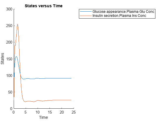
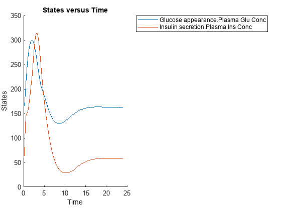
This example shows how to simulate the glucose-insulin responses for the normal and diabetic subjects.
Load the model of glucose-insulin response. For details about the model, see the Background section in Simulate the Glucose-Insulin Response.
sbioloadproject('insulindemo', 'm1')
The model contains different initial conditions stored in various variants.
variants = getvariant(m1);
Get the initial conditions for the type 2 diabetic patient.
type2 = variants(1)
type2 =
   SimBiology Variant - Type 2 diabetic (inactive)

   ContentIndex:     Type:        Name:             Property:           Value:
   1                 parameter    Plasma Volume ... Value               1.49
   2                 parameter    k1                Value               .042
   3                 parameter    k2                Value               .071
   4                 parameter    Plasma Volume ... Value               .04
   5                 parameter    m1                Value               .379
   6                 parameter    m2                Value               .673
   7                 parameter    m4                Value               .269
   8                 parameter    m5                Value               .0526
   9                 parameter    m6                Value               .8118
   10                parameter    Hepatic Extrac... Value               .6
   11                parameter    kmax              Value               .0465
   12                parameter    kmin              Value               .0076
   13                parameter    kabs              Value               .023
   14                parameter    kgri              Value               .0465
   15                parameter    f                 Value               .9
   16                parameter    a                 Value               6e-05
   17                parameter    b                 Value               .68
   18                parameter    c                 Value               .00023
   19                parameter    d                 Value               .09
   20                parameter    kp1               Value               3.09
   21                parameter    kp2               Value               .0007
   22                parameter    kp3               Value               .005
   23                parameter    kp4               Value               .0786
   24                parameter    ki                Value               .0066
   25                parameter    [Ins Ind Glu U... Value               1.0
   26                parameter    Vm0               Value               4.65
   27                parameter    Vmx               Value               .034
   28                parameter    Km                Value               466.21
   29                parameter    p2U               Value               .084
   30                parameter    K                 Value               .99
   31                parameter    alpha             Value               .013
   32                parameter    beta              Value               .05
   33                parameter    gamma             Value               .5
   34                parameter    ke1               Value               .0007
   35                parameter    ke2               Value               269.0
   36                parameter    Basal Plasma G... Value               164.18
   37                parameter    Basal Plasma I... Value               54.81
Suppress an informational warning that is issued during simulations.
warnSettings = warning('off','SimBiology:DimAnalysisNotDone_MatlabFcn_Dimensionless');
Create SimFunction objects to simulate the glucose-insulin response for the normal and diabetic subjects.
Specify an empty array
{}for the second input argument to denote that the model will be simulated using the base parameter values (that is, no parameter scanning will be performed).Specify the plasma glucose and insulin concentrations as responses (outputs of the function to be plotted).
Specify the species
Doseas the dosed species. This species represents the initial concentration of glucose at the start of the simulation.
normSim = createSimFunction(m1,{},...
             {'[Plasma Glu Conc]','[Plasma Ins Conc]'},'Dose')
normSim =
SimFunction
Parameters:
Name Value Type Units
____ _____ ____ _____
Observables:
Name Type Units
_____________________ ___________ _______________________
{'[Plasma Glu Conc]'} {'species'} {'milligram/deciliter'}
{'[Plasma Ins Conc]'} {'species'} {'picomole/liter' }
Dosed:
TargetName TargetDimension
__________ _____________________
{'Dose'} {'Mass (e.g., gram)'}
TimeUnits: hour
For the diabetic patient, specify the initial conditions using the variant type2.
diabSim = createSimFunction(m1,{},...
             {'[Plasma Glu Conc]','[Plasma Ins Conc]'},'Dose',type2)
diabSim =
SimFunction
Parameters:
Name Value Type Units
____ _____ ____ _____
Observables:
Name Type Units
_____________________ ___________ _______________________
{'[Plasma Glu Conc]'} {'species'} {'milligram/deciliter'}
{'[Plasma Ins Conc]'} {'species'} {'picomole/liter' }
Dosed:
TargetName TargetDimension
__________ _____________________
{'Dose'} {'Mass (e.g., gram)'}
TimeUnits: hour
Select a dose that represents a single meal of 78 grams of glucose at the start of the simulation.
singleMeal = sbioselect(m1,'Name','Single Meal');
Convert the dosing information to the table format.
mealTable = getTable(singleMeal);
Simulate the glucose-insulin response for a normal subject for 24 hours.
sbioplot(normSim([],24,mealTable));
Simulate the glucose-insulin response for a diabetic subject for 24 hours.
sbioplot(diabSim([],24,mealTable));
Perform a Scan Using Variants
Suppose you want to perform a parameter scan using an array of variants that contain different initial conditions for different insulin impairments. For example, the model m1 has variants that correspond to the low insulin sensitivity and high insulin sensitivity. You can simulate the model for both conditions via a single call to the SimFunction object.
Select the variants to scan.
varToScan = sbioselect(m1,'Name',...
                    {'Low insulin sensitivity','High insulin sensitivity'});
Check which model parameters are being stored in each variant.
varToScan(1)
ans =
   SimBiology Variant - Low insulin sensitivity (inactive)

   ContentIndex:     Type:        Name:             Property:           Value:
   1                 parameter    Vmx               Value               .0235
   2                 parameter    kp3               Value               .0045
varToScan(2)
ans =
   SimBiology Variant - High insulin sensitivity (inactive)

   ContentIndex:     Type:        Name:             Property:           Value:
   1                 parameter    Vmx               Value               .094
   2                 parameter    kp3               Value               .018
Both variants store alternate values for Vmx and kp3 parameters. You need to specify them as input parameters when you create a SimFunction object.
Create a SimFunction object to scan the variants.
variantScan = createSimFunction(m1,{'Vmx','kp3'},...
          {'[Plasma Glu Conc]','[Plasma Ins Conc]'},'Dose');
Simulate the model and plot the results. Run 1 include simulation results for the low insulin sensitivity and Run 2 for the high insulin sensitivity.
sbioplot(variantScan(varToScan,24,mealTable));
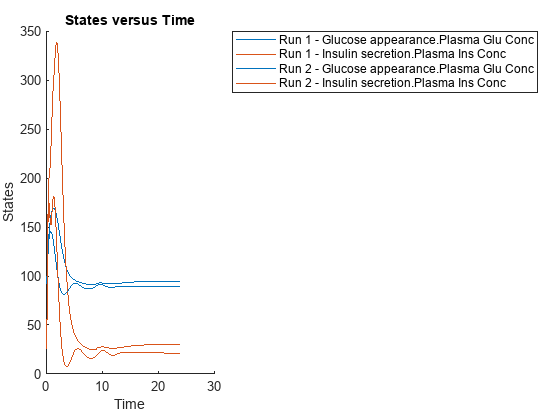
Low insulin sensitivity lead to increased and prolonged plasma glucose concentration.
Restore warning settings.
warning(warnSettings);
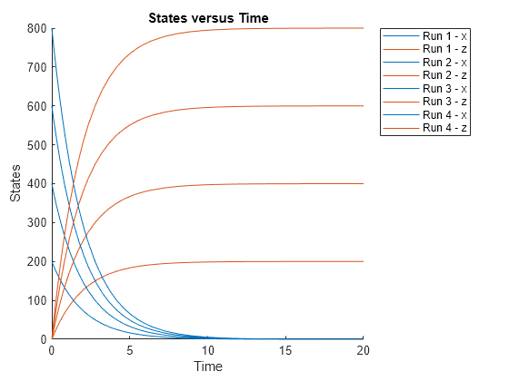
This example shows how to scan initial amounts of a species from a radioactive decay model with the first-order reaction , where x and z are species and c is the forward rate constant.
Load the sample project containing the radiodecay model m1.
sbioloadproject radiodecay;Create a SimFunction object f to scan initial amounts of species x.
f = createSimFunction(m1,{'x'},{'x','z'},[])f =
SimFunction
Parameters:
Name Value Type Units
_____ _____ ___________ ____________
{'x'} 1000 {'species'} {'molecule'}
Observables:
Name Type Units
_____ ___________ ____________
{'x'} {'species'} {'molecule'}
{'z'} {'species'} {'molecule'}
Dosed: None
TimeUnits: second
Define four different initial amounts of species x for scanning. The number of rows indicates the total number of simulations, and each simulation uses the parameter value specified in each row of the vector.
phi = [200; 400; 600; 800];
Run simulations until the stop time is 20 and plot the simulation results.
sbioplot(f(phi, 20));
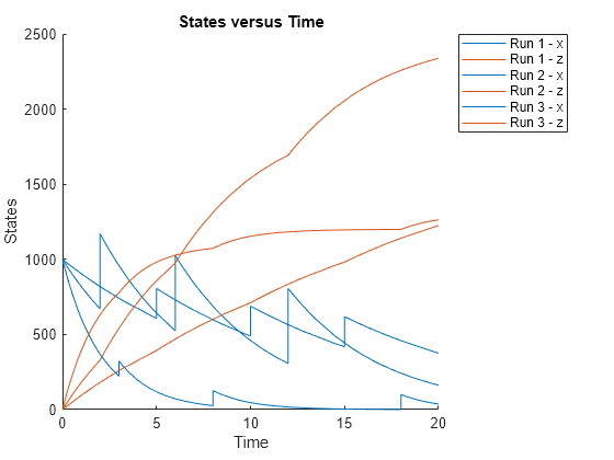
This example shows how to simulate and scan a parameter of a radiodecay model while a species is being dosed.
Load the sample project containing the radiodecay model m1.
sbioloadproject radiodecay;Create a SimFunction object f specifying parameter Reaction1.c to be scanned and species x as a dosed target.
f = createSimFunction(m1,{'Reaction1.c'},{'x','z'},{'x'});Define a scalar dose of amount 200 molecules given at three time points (5, 10, and 15 seconds).
dosetime = [5 10 15];
dose = [200 200 200];
u = table(dosetime', dose');
u.Properties.VariableNames = {'Time','Amount'};
u.Properties.VariableUnits = {'second','molecule'};
Define the parameter values for Reaction1.c to scan.
phi = [0.1 0.2 0.5]';
Simulate the model for 20 seconds and plot the results.
sbioplot(f(phi,20,u));

You can also specify different dose amounts at different times.
d1 = table(5,100);
d1.Properties.VariableNames = {'Time','Amount'};
d1.Properties.VariableUnits = {'second','molecule'};
d2 = table(10,300);
d2.Properties.VariableNames = {'Time','Amount'};
d2.Properties.VariableUnits = {'second','molecule'};
d3 = table(15,600);
d3.Properties.VariableNames = {'Time','Amount'};
d3.Properties.VariableUnits = {'second','molecule'};
Simulate the model using these doses and plot the results.
sbioplot(f(phi,20,{d1;d2;d3}));
You can also define a cell array of dose tables.
u = cell(3,1);
dosetime = [5 10 15];
dose = [200 200 200];
u{1} = table(dosetime',dose');
u{1}.Properties.VariableNames = {'Time','Amount'};
u{1}.Properties.VariableUnits = {'second','molecule'};
dosetime2 = [2 6 12];
dose2 = [500 500 500];
u{2} = table(dosetime2', dose2');
u{2}.Properties.VariableNames = {'Time','Amount'};
u{2}.Properties.VariableUnits = {'second','molecule'};
dosetime3 = [3 8 18];
dose3 = [100 100 100];
u{3} = table(dosetime3', dose3');
u{3}.Properties.VariableNames = {'Time','Amount'};
u{3}.Properties.VariableUnits = {'second','molecule'};
Simulate the model using the dose tables and plot results.
sbioplot(f(phi,20,u));
References
[1] Gillespie, D.T. (1977). Exact Stochastic Simulation of Coupled Chemical Reactions. The Journal of Physical Chemistry. 81(25), 2340–2361.
Version History
Introduced in R2014a
MATLAB Command
You clicked a link that corresponds to this MATLAB command:
Run the command by entering it in the MATLAB Command Window. Web browsers do not support MATLAB commands.
选择网站
选择网站以获取翻译的可用内容,以及查看当地活动和优惠。根据您的位置,我们建议您选择:。
您也可以从以下列表中选择网站:
如何获得最佳网站性能
选择中国网站(中文或英文)以获得最佳网站性能。其他 MathWorks 国家/地区网站并未针对您所在位置的访问进行优化。
美洲
- América Latina (Español)
- Canada (English)
- United States (English)
欧洲
- Belgium (English)
- Denmark (English)
- Deutschland (Deutsch)
- España (Español)
- Finland (English)
- France (Français)
- Ireland (English)
- Italia (Italiano)
- Luxembourg (English)
- Netherlands (English)
- Norway (English)
- Österreich (Deutsch)
- Portugal (English)
- Sweden (English)
- Switzerland
- United Kingdom (English)