plotData
Plot quantile summary of model simulations from global sensitivity analysis
Description
h = plotData(resultsObj)h.
h = plotData(resultsObj,Name,Value)
Examples
Load the tumor growth model.
sbioloadproject tumor_growth_vpop_sa.sbprojGet a variant with the estimated parameters and the dose to apply to the model.
v = getvariant(m1);
d = getdose(m1,'interval_dose');
Get the active configset and set the tumor weight as the response.
cs = getconfigset(m1);
cs.RuntimeOptions.StatesToLog = 'tumor_weight';
Simulate the model and plot the tumor growth profile.
sbioplot(sbiosimulate(m1,cs,v,d));

Perform global sensitivity analysis (GSA) on the model to find the model parameters that the tumor growth is sensitive to.
First, retrieve model parameters of interest that are involved in the pharmacodynamics of the tumor growth. Define the model response as the tumor weight.
modelParamNames = {'L0','L1','w0','k1','k2'};
outputName = 'tumor_weight';
Then perform GSA by computing the first- and total-order Sobol indices using sbiosobol. Set 'ShowWaitBar' to true to show the simulation progress. By default, the function uses 1000 parameter samples to compute the Sobol indices [1].
rng('default');
sobolResults = sbiosobol(m1,modelParamNames,outputName,Variants=v,Doses=d,ShowWaitBar=true)
sobolResults =
Sobol with properties:
Time: [444×1 double]
SobolIndices: [5×1 struct]
Variance: [444×1 table]
ParameterSamples: [1000×5 table]
Observables: {'[Tumor Growth].tumor_weight'}
SimulationInfo: [1×1 struct]
You can change the number of samples by specifying the 'NumberSamples' name-value pair argument. The function requires a total of (number of input parameters + 2) * NumberSamples model simulations.
Show the mean model response, the simulation results, and a shaded region covering 90% of the simulation results.
plotData(sobolResults,ShowMedian=true,ShowMean=false);
![Figure contains an axes object. The axes object with xlabel time, ylabel [Tumor Growth].tumor indexOf w baseline eight contains 12 objects of type line, patch. These objects represent model simulation, 90.0% region, median value.](../../examples/simbio/win64/PerformGSAByComputingFirstAndTotalSobolIndicesExample_02.png)
You can adjust the quantile region to a different percentage by specifying 'Alphas' for the lower and upper quantiles of all model responses. For instance, an alpha value of 0.1 plots a shaded region between the 100 * alpha and 100 * (1 - alpha) quantiles of all simulated model responses.
plotData(sobolResults,Alphas=0.1,ShowMedian=true,ShowMean=false);
![Figure contains an axes object. The axes object with xlabel time, ylabel [Tumor Growth].tumor indexOf w baseline eight contains 12 objects of type line, patch. These objects represent model simulation, 80.0% region, median value.](../../examples/simbio/win64/PerformGSAByComputingFirstAndTotalSobolIndicesExample_03.png)
Plot the time course of the first- and total-order Sobol indices.
h = plot(sobolResults);
% Resize the figure.
h.Position(:) = [100 100 1280 800];![Figure contains 12 axes objects. Axes object 1 with xlabel time, ylabel total variance contains an object of type line. Axes object 2 with xlabel time, ylabel fraction of unexplained variance contains 3 objects of type line. Axes object 3 with ylabel total order k2 contains 3 objects of type line. Axes object 4 with ylabel first order k2 contains 3 objects of type line. Axes object 5 with ylabel total order k1 contains 3 objects of type line. Axes object 6 with ylabel first order k1 contains 3 objects of type line. Axes object 7 with ylabel total order w0 contains 3 objects of type line. Axes object 8 with ylabel first order w0 contains 3 objects of type line. Axes object 9 with ylabel total order L1 contains 3 objects of type line. Axes object 10 with ylabel first order L1 contains 3 objects of type line. Axes object 11 with title sensitivity output [Tumor Growth].tumor_weight, ylabel total order L0 contains 3 objects of type line. Axes object 12 with title sensitivity output [Tumor Growth].tumor_weight, ylabel first order L0 contains 3 objects of type line.](../../examples/simbio/win64/PerformGSAByComputingFirstAndTotalSobolIndicesExample_04.png)
The first-order Sobol index of an input parameter gives the fraction of the overall response variance that can be attributed to variations in the input parameter alone. The total-order index gives the fraction of the overall response variance that can be attributed to any joint parameter variations that include variations of the input parameter.
From the Sobol indices plots, parameters L1 and w0 seem to be the most sensitive parameters to the tumor weight before the dose was applied at t = 7. But after the dose is applied, k1 and k2 become more sensitive parameters and contribute most to the after-dosing stage of the tumor weight. The total variance plot also shows a larger variance for the after-dose stage at t > 35 than for the before-dose stage of the tumor growth, indicating that k1 and k2 might be more important parameters to investigate further. The fraction of unexplained variance shows some variance at around t = 33, but the total variance plot shows little variance at t = 33, meaning the unexplained variance could be insignificant. The fraction of unexplained variance is calculated as 1 - (sum of all the first-order Sobol indices), and the total variance is calculated using var(response), where response is the model response at every time point.
You can also display the magnitudes of the sensitivities in a bar plot. Darker colors mean that those values occur more often over the whole time course.
bar(sobolResults);
![Figure contains an axes object. The axes object with title sensitivity output [Tumor Growth].tumor_weight, xlabel Sobol Index, ylabel sensitivity input contains 22 objects of type patch, line. These objects represent first order, total order.](../../examples/simbio/win64/PerformGSAByComputingFirstAndTotalSobolIndicesExample_05.png)
You can specify more samples to increase the accuracy of the Sobol indices, but the simulation can take longer to finish. Use addsamples to add more samples. For example, if you specify 1500 samples, the function performs 1500 * (2 + number of input parameters) simulations.
gsaMoreSamples = addsamples(gsaResults,1500)
The SimulationInfo property of the result object contains various information for computing the Sobol indices. For instance, the model simulation data (SimData) for each simulation using a set of parameter samples is stored in the SimData field of the property. This field is an array of SimData objects.
sobolResults.SimulationInfo.SimData
   SimBiology SimData Array : 1000-by-7

   Index:    Name:         ModelName:         DataCount:
   1           -           Tumor Growth Model 1
   2           -           Tumor Growth Model 1
   3           -           Tumor Growth Model 1
   ...
   7000        -           Tumor Growth Model 1
You can find out if any model simulation failed during the computation by checking the ValidSample field of SimulationInfo. In this example, the field shows no failed simulation runs.
all(sobolResults.SimulationInfo.ValidSample)
ans = 1×7 logical array

   1   1   1   1   1   1   1
SimulationInfo.ValidSample is a table of logical values. It has the same size as SimulationInfo.SimData. If ValidSample indicates that any simulations failed, you can get more information about those simulation runs and the samples used for those runs by extracting information from the corresponding column of SimulationInfo.SimData. Suppose that the fourth column contains one or more failed simulation runs. Get the simulation data and sample values used for that simulation using getSimulationResults.
[samplesUsed,sd,validruns] = getSimulationResults(sobolResults,4);
You can add custom expressions as observables and compute Sobol indices for the added observables. For example, you can compute the Sobol indices for the maximum tumor weight by defining a custom expression as follows.
% Suppress an information warning that is issued during simulation.
warnSettings = warning('off', 'SimBiology:sbservices:SB_DIMANALYSISNOTDONE_MATLABFCN_UCON');
% Add the observable expression.
sobolObs = addobservable(sobolResults,'Maximum tumor_weight','max(tumor_weight)','Units','gram');
Plot the computed simulation results showing the 90% quantile region.
h2 = plotData(sobolObs,ShowMedian=true,ShowMean=false);
h2.Position(:) = [100 100 1280 800];
![Figure contains 2 axes objects. Axes object 1 with ylabel Maximum tumor_weight contains 12 objects of type line, patch. One or more of the lines displays its values using only markers These objects represent model simulation, 90.0% region, median value. Axes object 2 with xlabel time, ylabel [Tumor Growth].tumor_weight contains 12 objects of type line, patch. These objects represent model simulation, 90.0% region, median value.](../../examples/simbio/win64/PerformGSAByComputingFirstAndTotalSobolIndicesExample_06.png)
You can also remove the observable by specifying its name.
gsaNoObs = removeobservable(sobolObs,'Maximum tumor_weight');Restore the warning settings.
warning(warnSettings);
Load the target-mediated drug disposition (TMDD) model.
sbioloadproject tmdd_with_TO.sbprojGet the active configset and set the target occupancy (TO) as the response.
cs = getconfigset(m1);
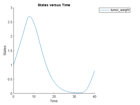
cs.RuntimeOptions.StatesToLog = 'TO';Simulate the model and plot the TO profile.
sbioplot(sbiosimulate(m1,cs));
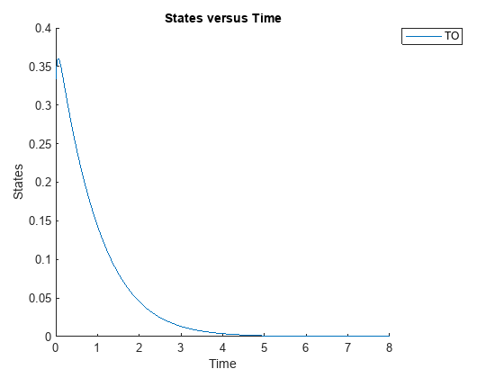
Define an exposure (area under the curve of the TO profile) threshold for the target occupancy.
classifier = 'trapz(time,TO) <= 0.1';Perform MPGSA to find sensitive parameters with respect to the TO. Vary the parameter values between predefined bounds to generate 10,000 parameter samples.
% Suppress an information warning that is issued during simulation.
warnSettings = warning('off', 'SimBiology:sbservices:SB_DIMANALYSISNOTDONE_MATLABFCN_UCON');
rng(0,'twister'); % For reproducibility
params = {'kel','ksyn','kdeg','km'};
bounds = [0.1, 1;
          0.1, 1;
          0.1, 1;
          0.1, 1];
mpgsaResults = sbiompgsa(m1,params,classifier,Bounds=bounds,NumberSamples=10000)
mpgsaResults =
  MPGSA with properties:

                    Classifiers: {'trapz(time,TO) <= 0.1'}
    KolmogorovSmirnovStatistics: [4×1 table]
                       ECDFData: {4×4 cell}
              SignificanceLevel: 0.0500
                        PValues: [4×1 table]
              SupportHypothesis: [10000×1 table]
               ParameterSamples: [10000×4 table]
                    Observables: {'TO'}
                 SimulationInfo: [1×1 struct]
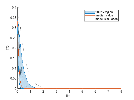
Plot the quantiles of the simulated model response.
plotData(mpgsaResults,ShowMedian=true,ShowMean=false);
Plot the empirical cumulative distribution functions (eCDFs) of the accepted and rejected samples. Except for km, none of the parameters shows a significant difference in the eCDFs for the accepted and rejected samples. The km plot shows a large Kolmogorov-Smirnov (K-S) distance between the eCDFs of the accepted and rejected samples. The K-S distance is the maximum absolute distance between two eCDFs curves.
h = plot(mpgsaResults);
% Resize the figure.
pos = h.Position(:);
h.Position(:) = [pos(1) pos(2) pos(3)*2 pos(4)*2];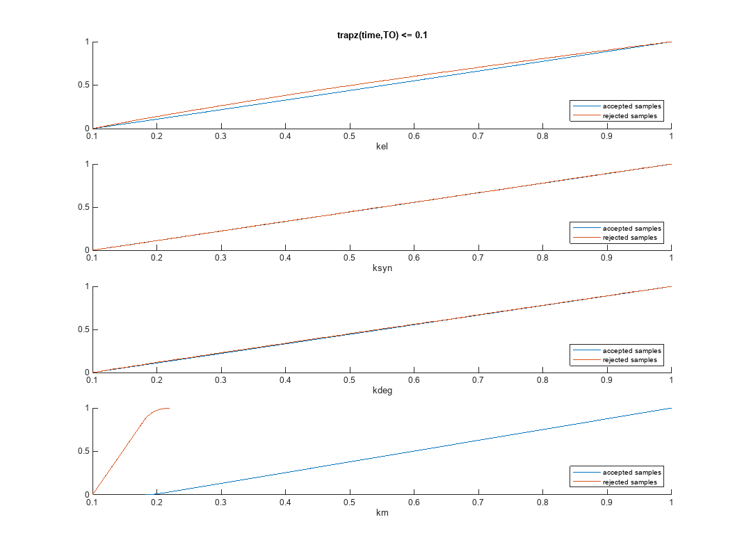
To compute the K-S distance between the two eCDFs, SimBiology uses a two-sided test based on the null hypothesis that the two distributions of accepted and rejected samples are equal. See kstest2 (Statistics and Machine Learning Toolbox) for details. If the K-S distance is large, then the two distributions are different, meaning that the classification of the samples is sensitive to variations in the input parameter. On the other hand, if the K-S distance is small, then variations in the input parameter do not affect the classification of samples. The results suggest that the classification is insensitive to the input parameter. To assess the significance of the K-S statistic rejecting the null-hypothesis, you can examine the p-values.
bar(mpgsaResults)
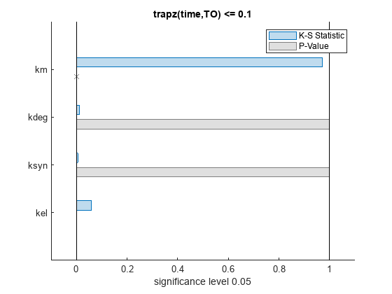
The bar plot shows two bars for each parameter: one for the K-S distance (K-S statistic) and another for the corresponding p-value. You reject the null hypothesis if the p-value is less than the significance level. A cross (x) is shown for any p-value that is almost 0. You can see the exact p-value corresponding to each parameter.
[mpgsaResults.ParameterSamples.Properties.VariableNames',mpgsaResults.PValues]
ans=4×2 table
      Var1      trapz(time,TO) <= 0.1
    ________    _____________________

    {'kel' }          0.0021877
    {'ksyn'}                  1
    {'kdeg'}            0.99983
    {'km'  }                  0
The p-values of km and kel are less than the significance level (0.05), supporting the alternative hypothesis that the accepted and rejected samples come from different distributions. In other words, the classification of the samples is sensitive to km and kel but not to other parameters (kdeg and ksyn).
You can also plot the histograms of accepted and rejected samples. The historgrams let you see trends in the accepted and rejected samples. In this example, the histogram of km shows that there are more accepted samples for larger km values, while the kel histogram shows that there are fewer rejected samples as kel increases.
h2 = histogram(mpgsaResults);
% Resize the figure.
pos = h2.Position(:);
h2.Position(:) = [pos(1) pos(2) pos(3)*2 pos(4)*2];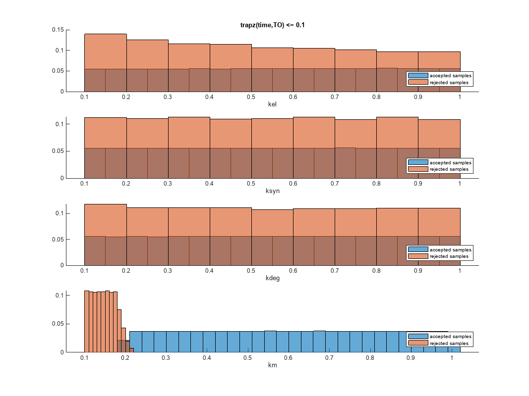
Restore the warning settings.
warning(warnSettings);
Load the tumor growth model.
sbioloadproject tumor_growth_vpop_sa.sbprojGet a variant with estimated parameters and the dose to apply to the model.
v = getvariant(m1);
d = getdose(m1,'interval_dose');
Get the active configset and set the tumor weight as the response.
cs = getconfigset(m1);
cs.RuntimeOptions.StatesToLog = 'tumor_weight';
Simulate the model and plot the tumor growth profile.
sbioplot(sbiosimulate(m1,cs,v,d));
Perform global sensitivity analysis (GSA) on the model to find the model parameters that the tumor growth is sensitive to.
First, define model parameters of interest, which are involved in the pharmacodynamics of the tumor growth. Define the model response as the tumor weight.
modelParamNames = {'L0','L1','w0','k1'};
outputName = 'tumor_weight';
Then perform GSA by computing the elementary effects using sbioelementaryeffects. Use 100 as the number of samples and set ShowWaitBar to true to show the simulation progress.
rng('default');
eeResults = sbioelementaryeffects(m1,modelParamNames,outputName,Variants=v,Doses=d,NumberSamples=100,ShowWaitbar=true);
Show the median model response, the simulation results, and a shaded region covering 90% of the simulation results.
plotData(eeResults,ShowMedian=true,ShowMean=false);
![Figure contains an axes object. The axes object with xlabel time, ylabel [Tumor Growth].tumor indexOf w baseline eight contains 12 objects of type line, patch. These objects represent model simulation, 90.0% region, median value.](../../examples/simbio/win64/PerformGSAByComputingElementaryEffectsExample_02.png)
You can adjust the quantile region to a different percentage by specifying Alphas for the lower and upper quantiles of all model responses. For instance, an alpha value of 0.1 plots a shaded region between the 100*alpha and 100*(1-alpha) quantiles of all simulated model responses.
plotData(eeResults,Alphas=0.1,ShowMedian=true,ShowMean=false);
![Figure contains an axes object. The axes object with xlabel time, ylabel [Tumor Growth].tumor indexOf w baseline eight contains 12 objects of type line, patch. These objects represent model simulation, 80.0% region, median value.](../../examples/simbio/win64/PerformGSAByComputingElementaryEffectsExample_03.png)
Plot the time course of the means and standard deviations of the elementary effects.
h = plot(eeResults);
% Resize the figure.
h.Position(:) = [100 100 1280 800];![Figure contains 8 axes objects. Axes object 1 with xlabel time, ylabel std. of effects k1 contains an object of type line. Axes object 2 with xlabel time, ylabel mean of effects k1 contains an object of type line. Axes object 3 with ylabel std. of effects w0 contains an object of type line. Axes object 4 with ylabel mean of effects w0 contains an object of type line. Axes object 5 with ylabel std. of effects L1 contains an object of type line. Axes object 6 with ylabel mean of effects L1 contains an object of type line. Axes object 7 with title sensitivity output [Tumor Growth].tumor_weight, ylabel std. of effects L0 contains an object of type line. Axes object 8 with title sensitivity output [Tumor Growth].tumor_weight, ylabel mean of effects L0 contains an object of type line.](../../examples/simbio/win64/PerformGSAByComputingElementaryEffectsExample_04.png)
The mean of effects explains whether variations in input parameter values have any effect on the tumor weight response. The standard deviation of effects explains whether the sensitivity change is dependent on the location in the parameter domain.
From the mean of effects plots, parameters L1 and w0 seem to be the most sensitive parameters to the tumor weight before the dose is applied at t = 7. But, after the dose is applied, k1 and L0 become more sensitive parameters and contribute most to the after-dosing stage of the tumor weight. The plots of standard deviation of effects show more deviations for the larger parameter values in the later stage (t > 35) than for the before-dose stage of the tumor growth.
You can also display the magnitudes of the sensitivities in a bar plot. Each color shading represents a histogram representing values at different times. Darker colors mean that those values occur more often over the whole time course.
bar(eeResults);
![Figure contains an axes object. The axes object with title sensitivity output [Tumor Growth].tumor_weight, xlabel elementary effects, ylabel sensitivity input contains 18 objects of type patch, line. These objects represent mean, standard deviation.](../../examples/simbio/win64/PerformGSAByComputingElementaryEffectsExample_05.png)
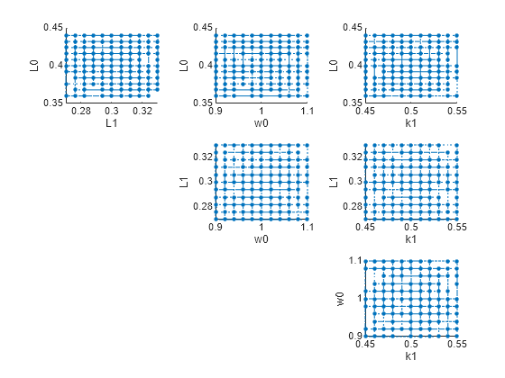
You can also plot the parameter grids and samples used to compute the elementary effects.
plotGrid(eeResults)
You can specify more samples to increase the accuracy of the elementary effects, but the simulation can take longer to finish. Use addsamples to add more samples.
eeResults2 = addsamples(eeResults,200);
The SimulationInfo property of the result object contains various information for computing the elementary effects. For instance, the model simulation data (SimData) for each simulation using a set of parameter samples is stored in the SimData field of the property. This field is an array of SimData objects.
eeResults2.SimulationInfo.SimData
   SimBiology SimData Array : 1500-by-1

   Index:    Name:         ModelName:         DataCount:
   1           -           Tumor Growth Model 1
   2           -           Tumor Growth Model 1
   3           -           Tumor Growth Model 1
   ...
   1500        -           Tumor Growth Model 1
You can find out if any model simulation failed during the computation by checking the ValidSample field of SimulationInfo. In this example, the field shows no failed simulation runs.
all(eeResults2.SimulationInfo.ValidSample)
ans = logical
   1
You can add custom expressions as observables and compute the elementary effects of the added observables. For example, you can compute the effects for the maximum tumor weight by defining a custom expression as follows.
% Suppress an information warning that is issued.
warnSettings = warning('off', 'SimBiology:sbservices:SB_DIMANALYSISNOTDONE_MATLABFCN_UCON');
% Add the observable expression.
eeObs = addobservable(eeResults2,'Maximum tumor_weight','max(tumor_weight)','Units','gram');
Plot the computed simulation results showing the 90% quantile region.
h2 = plotData(eeObs,ShowMedian=true,ShowMean=false);
h2.Position(:) = [100 100 1500 800];
![Figure contains 2 axes objects. Axes object 1 with ylabel Maximum tumor_weight contains 12 objects of type line, patch. One or more of the lines displays its values using only markers These objects represent model simulation, 90.0% region, median value. Axes object 2 with xlabel time, ylabel [Tumor Growth].tumor_weight contains 12 objects of type line, patch. These objects represent model simulation, 90.0% region, median value.](../../examples/simbio/win64/PerformGSAByComputingElementaryEffectsExample_07.png)
You can also remove the observable by specifying its name.
eeNoObs = removeobservable(eeObs,'Maximum tumor_weight');Restore the warning settings.
warning(warnSettings);
Input Arguments
Name-Value Arguments
Output Arguments
References
[1] Saltelli, Andrea, Paola Annoni, Ivano Azzini, Francesca Campolongo, Marco Ratto, and Stefano Tarantola. “Variance Based Sensitivity Analysis of Model Output. Design and Estimator for the Total Sensitivity Index.” Computer Physics Communications 181, no. 2 (February 2010): 259–70. https://doi.org/10.1016/j.cpc.2009.09.018.
[2] Tiemann, Christian A., Joep Vanlier, Maaike H. Oosterveer, Albert K. Groen, Peter A. J. Hilbers, and Natal A. W. van Riel. “Parameter Trajectory Analysis to Identify Treatment Effects of Pharmacological Interventions.” Edited by Scott Markel. PLoS Computational Biology 9, no. 8 (August 1, 2013): e1003166. https://doi.org/10.1371/journal.pcbi.1003166.
[3] Morris, Max D. “Factorial Sampling Plans for Preliminary Computational Experiments.” Technometrics 33, no. 2 (May 1991): 161–74.
[4] Sohier, Henri, Jean-Loup Farges, and Helene Piet-Lahanier. “Improvement of the Representativity of the Morris Method for Air-Launch-to-Orbit Separation.” IFAC Proceedings Volumes 47, no. 3 (2014): 7954–59.