SimFunctionSensitivity object

This example shows how to calculate the local sensitivities of some species in the Lotka-Volterra model using the SimFunctionSensitivity object.

Load the sample project.

sbioloadproject lotka;

Define the input parameters.

params = {'Reaction1.c1', 'Reaction2.c2'};

Define the observed species, which are the outputs of simulation.

observables  = {'y1', 'y2'};

Create a SimFunctionSensitivity object. Set the sensitivity output factors to all species (y1 and y2) specified in the observables argument and input factors to those in the params argument (c1 and c2) by setting the name-value pair argument to 'all'.

f = createSimFunction(m1,params,observables,[],'SensitivityOutputs','all','SensitivityInputs','all','SensitivityNormalization','Full')

f = 
SimFunction

Parameters:

          Name          Value        Type     
    ________________    _____    _____________

    {'Reaction1.c1'}      10     {'parameter'}
    {'Reaction2.c2'}    0.01     {'parameter'}

Observables: 

     Name        Type    
    ______    ___________

    {'y1'}    {'species'}
    {'y2'}    {'species'}

Dosed: None

Sensitivity Input Factors: 

          Name              Type     
    ________________    _____________

    {'Reaction1.c1'}    {'parameter'}
    {'Reaction2.c2'}    {'parameter'}

Sensitivity Output Factors: 

     Name        Type    
    ______    ___________

    {'y1'}    {'species'}
    {'y2'}    {'species'}

Sensitivity Normalization: 

Full

Calculate sensitivities by executing the object with c1 and c2 set to 10 and 0.1, respectively. Set the output times from 1 to 10. t contains time points, y contains simulation data, and sensMatrix is the sensitivity matrix containing sensitivities of y1 and y2 with respect to c1 and c2.

[t,y,sensMatrix] = f([10,0.1],[],[],1:10);

Retrieve the sensitivity information at time point 5.

temp = sensMatrix{:};
sensMatrix2 = temp(t{:}==5,:,:);
sensMatrix2 = squeeze(sensMatrix2)

sensMatrix2 = 2×2

   37.6987   -6.8447
  -40.2791    5.8225

The rows of sensMatrix2 represent the output factors (y1 and y2). The columns represent the input factors (c1 and c2).

Set the stop time to 15, without specifying the output times. In this case, the output times are the solver time points by default.

sd = f([10,0.1],15);

Retrieve the calculated sensitivities from the SimData object sd.

[t,y,outputs,inputs] = getsensmatrix(sd);

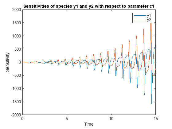
Plot the sensitivities of species y1 and y2 with respect to c1.

figure;
plot(t,y(:,:,1));
legend(outputs);
title('Sensitivities of species y1 and y2 with respect to parameter c1');
xlabel('Time');
ylabel('Sensitivity');

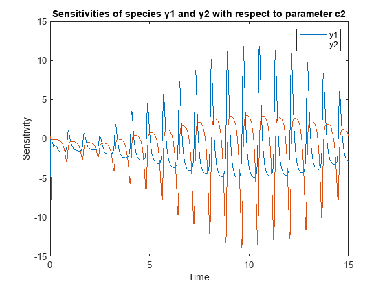
Plot the sensitivities of species y1 and y2 with respect to c2.

figure;
plot(t,y(:,:,2));
legend(outputs);
title('Sensitivities of species y1 and y2 with respect to parameter c2');
xlabel('Time');
ylabel('Sensitivity');

Alternatively, you can use sbioplot.

sbioplot(sd);

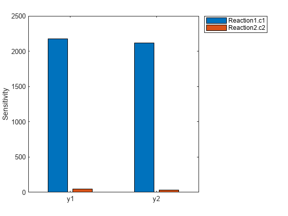
You can also plot the sensitivity matrix using the time integral for the calculated sensitivities of y1 and y2. The plot indicates y1 and y2 are more sensitive to c1 than c2.

[~, in, out] = size(y);
result = zeros(in, out);
for i = 1:in
    for j = 1:out
        result(i,j) = trapz(t(:),abs(y(:,i,j)));
    end
end
figure;
hbar = bar(result);
haxes = hbar(1).Parent;
haxes.XTick = 1:length(outputs);
haxes.XTickLabel = outputs;
legend(inputs,'Location','NorthEastOutside');
ylabel('Sensitivity');