createSimFunction

Create SimFunction object

Syntax

F = createSimFunction(model,params,observables,dosed)

F = createSimFunction(model,params,observables,dosed,variants)

F = createSimFunction(___,Name,Value)

Description

F = createSimFunction(model,params,observables,dosed) creates a SimFunction object F that you can execute like a function handle. The params and observables arguments define the inputs and outputs of the function F when it is executed, and dosed defines the dosing information of species. See SimFunction object for details on how to execute F.

Note

Active doses and variants of the model are ignored when F is executed.
F is immutable after it is created.
F is automatically accelerated at the first function execution unless you set AutoAccelerate to false. Manually accelerate the object if you want it accelerated in your deployment applications.

example

F = createSimFunction(model,params,observables,dosed,variants) creates a SimFunction object, applying the values stored in variants, a vector of variant objects, as the model baseline values.

example

F = createSimFunction(___,Name,Value) uses additional options specified by one or more Name,Value pair arguments.

example

Examples

collapse all

Create a SimFunction Object

Open Live Script

This example uses a radioactive decay model with the first-order reaction $\frac{d z}{d t} = c \cdot x$ , where x and z are species and c is the forward rate constant.

Load the sample project containing the radioactive decay model m1.

sbioloadproject radiodecay;

Create a SimFunction, specifying the parameter Reaction1.c to be scanned, and species x as the output of the function with no dosed species.

f = createSimFunction(m1, 'Reaction1.c','x', [])

f = 
SimFunction

Parameters:

         Name          Value        Type            Units    
    _______________    _____    _____________    ____________

    {'Reaction1.c'}     0.5     {'parameter'}    {'1/second'}

Observables: 

    Name        Type           Units    
    _____    ___________    ____________

    {'x'}    {'species'}    {'molecule'}

Dosed: None

TimeUnits: second

If the UnitConversion option was set to false when the SimFunction object f was created, the table does not display the units of the model quantities.

To illustrate this, first set the UnitConversion option to false.

cs = getconfigset(m1);
cs.CompileOptions.UnitConversion = false;

Create the SimFunction object as before and note that the variable named Units disappears.

f = createSimFunction(m1, {'Reaction1.c'},{'x'}, [])

f = 
SimFunction

Parameters:

         Name          Value        Type     
    _______________    _____    _____________

    {'Reaction1.c'}     0.5     {'parameter'}

Observables: 

    Name        Type    
    _____    ___________

    {'x'}    {'species'}

Dosed: None

If any of the species in the model is being dosed, specify the names of dosed species as the last argument. For example, if the species x is being dosed, specify it as the last argument.

f = createSimFunction(m1, {'Reaction1.c'},{'x'}, 'x')

f = 
SimFunction

Parameters:

         Name          Value        Type     
    _______________    _____    _____________

    {'Reaction1.c'}     0.5     {'parameter'}

Observables: 

    Name        Type    
    _____    ___________

    {'x'}    {'species'}

Dosed: 

    TargetName
    __________

      {'x'}

Once the SimFunction object is created, you can execute it like a function handle and perform parameter scans (in parallel if Parallel Computing Toolbox™ is available), Monte Carlo simulations, and scans with multiple or vectorized doses. See SimFunction for more examples.

Create a SimFunction Object with Dosing Information

Open Live Script

This example creates a SimFunction object with dosing information using a RepeatDose or ScheduleDose object or a vector of these objects. However, if any dose object contains data such as StartTime, Amount, and Rate, such data are ignored, and a warning is issued. Only data, if available, used are TargetName, LagParameterName, and DurationParameterName of the dose object.

Load the sample project containing the radioactive decay model m1.

sbioloadproject radiodecay;

Create a RepeatDose object and specify its properties.

rdose = sbiodose('rd');
rdose.TargetName = 'x';
rdose.StartTime = 5;
rdose.TimeUnits = 'second';
rdose.Amount = 300;
rdose.AmountUnits = 'molecule';
rdose.Rate = 1;
rdose.RateUnits = 'molecule/second';
rdose.Interval = 100;
rdose.RepeatCount = 2;

Add a lag parameter and duration parameter to the model.

lagPara = addparameter(m1,'lp');
lagPara.Value = 1;
lagPara.ValueUnits = 'second';
duraPara = addparameter(m1,'dp');
duraPara.Value = 1;
duraPara.ValueUnits = 'second';

Set these parameters to the dose object.

rdose.LagParameterName = 'lp';
rdose.DurationParameterName = 'dp';

Create a SimFunction object f using the RepeatDose object rdose that you just created. Turn off the information warning that is issued during simulation because the rdose object contains data (StartTime, Amount, Rate) that are ignored by the createSimFunction method.

warning('off','SimBiology:SimFunction:DOSES_NOT_EMPTY');
f = createSimFunction(m1,{'Reaction1.c'},{'x','z'},rdose)

f = 
SimFunction

Parameters:

         Name          Value        Type            Units    
    _______________    _____    _____________    ____________

    {'Reaction1.c'}     0.5     {'parameter'}    {'1/second'}

Observables: 

    Name        Type           Units    
    _____    ___________    ____________

    {'x'}    {'species'}    {'molecule'}
    {'z'}    {'species'}    {'molecule'}

Dosed: 

    TargetName              TargetDimension              DurationParameterName    DurationParameterValue    DurationParameterUnits    LagParameterName    LagParameterValue    LagParameterUnits
    __________    ___________________________________    _____________________    ______________________    ______________________    ________________    _________________    _________________

      {'x'}       {'Amount (e.g., mole or molecule)'}           {'dp'}                      1                     {'second'}               {'lp'}                 1               {'second'}    


TimeUnits: second

Turn the warning back on.

warning('on','SimBiology:SimFunction:DOSES_NOT_EMPTY');

Scan Parameters of the Lotka-Volterra Model

Open Live Script

This example shows how to execute different signatures of the SimFunction to simulate and scan parameters of the Lotka-Volterra (predator-prey) model described by Gillespie [1].

Load the sample project containing the model m1.

sbioloadproject lotka;

Create a SimFunction object f with c1 and c2 as input parameters to be scanned, and y1 and y2 as the output of the function with no dosed species.

f = createSimFunction(m1,{'Reaction1.c1', 'Reaction2.c2'},{'y1', 'y2'}, [])

f = 
SimFunction

Parameters:

          Name          Value        Type     
    ________________    _____    _____________

    {'Reaction1.c1'}      10     {'parameter'}
    {'Reaction2.c2'}    0.01     {'parameter'}

Observables: 

     Name        Type    
    ______    ___________

    {'y1'}    {'species'}
    {'y2'}    {'species'}

Dosed: None

Define an input matrix that contains values for each parameter (c1 and c2) for each simulation. The number of rows indicates the total number of simulations, and each simulation uses the parameter values specified in each row.

phi = [10 0.01; 10 0.02];

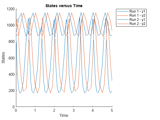
Run simulations until the stop time is 5 and plot the simulation results.

sbioplot(f(phi, 5));

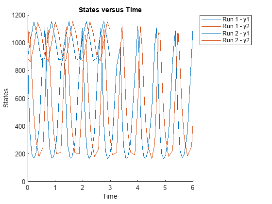
Figure contains an axes object. The axes object with title States versus Time, xlabel Time, ylabel States contains 4 objects of type line. These objects represent Run 1 - y1, Run 1 - y2, Run 2 - y1, Run 2 - y2.

You can also specify a vector of different stop times for each simulation.

t_stop = [3;6];
sbioplot(f(phi, t_stop));

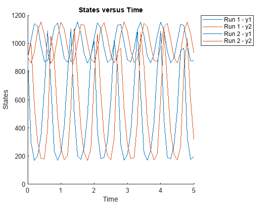
Next, specify the output times as a vector.

t_output = 0:0.1:5;
sbioplot(f(phi,[],[],t_output));

Specify output times as a cell array of vectors.

t_output = {0:0.01:3, 0:0.2:6};
sbioplot(f(phi, [], [], t_output));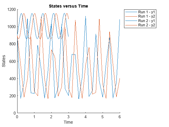

Calculate Local Sensitivities Using `SimFunctionSensitivity` Object

Open Live Script

This example shows how to calculate the local sensitivities of some species in the Lotka-Volterra model using the SimFunctionSensitivity object.

Load the sample project.

sbioloadproject lotka;

Define the input parameters.

params = {'Reaction1.c1', 'Reaction2.c2'};

Define the observed species, which are the outputs of simulation.

observables  = {'y1', 'y2'};

Create a SimFunctionSensitivity object. Set the sensitivity output factors to all species (y1 and y2) specified in the observables argument and input factors to those in the params argument (c1 and c2) by setting the name-value pair argument to 'all'.

f = createSimFunction(m1,params,observables,[],'SensitivityOutputs','all','SensitivityInputs','all','SensitivityNormalization','Full')

f = 
SimFunction

Parameters:

          Name          Value        Type     
    ________________    _____    _____________

    {'Reaction1.c1'}      10     {'parameter'}
    {'Reaction2.c2'}    0.01     {'parameter'}

Observables: 

     Name        Type    
    ______    ___________

    {'y1'}    {'species'}
    {'y2'}    {'species'}

Dosed: None

Sensitivity Input Factors: 

          Name              Type     
    ________________    _____________

    {'Reaction1.c1'}    {'parameter'}
    {'Reaction2.c2'}    {'parameter'}

Sensitivity Output Factors: 

     Name        Type    
    ______    ___________

    {'y1'}    {'species'}
    {'y2'}    {'species'}

Sensitivity Normalization: 

Full

Calculate sensitivities by executing the object with c1 and c2 set to 10 and 0.1, respectively. Set the output times from 1 to 10. t contains time points, y contains simulation data, and sensMatrix is the sensitivity matrix containing sensitivities of y1 and y2 with respect to c1 and c2.

[t,y,sensMatrix] = f([10,0.1],[],[],1:10);

Retrieve the sensitivity information at time point 5.

temp = sensMatrix{:};
sensMatrix2 = temp(t{:}==5,:,:);
sensMatrix2 = squeeze(sensMatrix2)

sensMatrix2 = 2×2

   37.6987   -6.8447
  -40.2791    5.8225

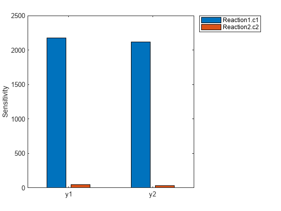
The rows of sensMatrix2 represent the output factors (y1 and y2). The columns represent the input factors (c1 and c2).

$s e n s M a t r i x 2 = [\begin{array}{cccccccccccccccccccc} \begin{array}{cccccccccccccccccccc} \frac{\partial y 1}{\partial c 1} \\ \frac{\partial y 2}{\partial c 1} \end{array} & \begin{array}{cccccccccccccccccccc} \frac{\partial y 1}{\partial c 2} \\ \frac{\partial y 2}{\partial c 2} \end{array} \end{array}]$

Set the stop time to 15, without specifying the output times. In this case, the output times are the solver time points by default.

sd = f([10,0.1],15);

Retrieve the calculated sensitivities from the SimData object sd.

[t,y,outputs,inputs] = getsensmatrix(sd);

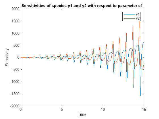
Plot the sensitivities of species y1 and y2 with respect to c1.

figure;
plot(t,y(:,:,1));
legend(outputs);
title('Sensitivities of species y1 and y2 with respect to parameter c1');
xlabel('Time');
ylabel('Sensitivity');

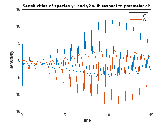
Figure contains an axes object. The axes object with title Sensitivities of species y1 and y2 with respect to parameter c1, xlabel Time, ylabel Sensitivity contains 2 objects of type line. These objects represent y1, y2.

Plot the sensitivities of species y1 and y2 with respect to c2.

figure;
plot(t,y(:,:,2));
legend(outputs);
title('Sensitivities of species y1 and y2 with respect to parameter c2');
xlabel('Time');
ylabel('Sensitivity');

Figure contains an axes object. The axes object with title Sensitivities of species y1 and y2 with respect to parameter c2, xlabel Time, ylabel Sensitivity contains 2 objects of type line. These objects represent y1, y2.

Alternatively, you can use sbioplot.

sbioplot(sd);

Figure contains an axes object. The axes object with title States versus Time, xlabel Time, ylabel States contains 6 objects of type line. These objects represent y1, y2, d[y1]/d[Reaction1.c1], d[y2]/d[Reaction1.c1], d[y1]/d[Reaction2.c2], d[y2]/d[Reaction2.c2].

You can also plot the sensitivity matrix using the time integral for the calculated sensitivities of y1 and y2. The plot indicates y1 and y2 are more sensitive to c1 than c2.

[~, in, out] = size(y);
result = zeros(in, out);
for i = 1:in
    for j = 1:out
        result(i,j) = trapz(t(:),abs(y(:,i,j)));
    end
end
figure;
hbar = bar(result);
haxes = hbar(1).Parent;
haxes.XTick = 1:length(outputs);
haxes.XTickLabel = outputs;
legend(inputs,'Location','NorthEastOutside');
ylabel('Sensitivity');

Figure contains an axes object. The axes object with ylabel Sensitivity contains 2 objects of type bar. These objects represent Reaction1.c1, Reaction2.c2.

Simulate Model of Glucose-Insulin Response with Different Initial Conditions

Open Live Script

This example shows how to simulate the glucose-insulin responses for the normal and diabetic subjects.

Load the model of glucose-insulin response. For details about the model, see the Background section in Simulate the Glucose-Insulin Response.

sbioloadproject('insulindemo', 'm1')

The model contains different initial conditions stored in various variants.

variants = getvariant(m1);

Get the initial conditions for the type 2 diabetic patient.

type2 = variants(1)

type2 = 
   SimBiology Variant - Type 2 diabetic (inactive)

   ContentIndex:     Type:        Name:             Property:           Value:
   1                 parameter    Plasma Volume ... Value               1.49
   2                 parameter    k1                Value               .042
   3                 parameter    k2                Value               .071
   4                 parameter    Plasma Volume ... Value               .04
   5                 parameter    m1                Value               .379
   6                 parameter    m2                Value               .673
   7                 parameter    m4                Value               .269
   8                 parameter    m5                Value               .0526
   9                 parameter    m6                Value               .8118
   10                parameter    Hepatic Extrac... Value               .6
   11                parameter    kmax              Value               .0465
   12                parameter    kmin              Value               .0076
   13                parameter    kabs              Value               .023
   14                parameter    kgri              Value               .0465
   15                parameter    f                 Value               .9
   16                parameter    a                 Value               6e-05
   17                parameter    b                 Value               .68
   18                parameter    c                 Value               .00023
   19                parameter    d                 Value               .09
   20                parameter    kp1               Value               3.09
   21                parameter    kp2               Value               .0007
   22                parameter    kp3               Value               .005
   23                parameter    kp4               Value               .0786
   24                parameter    ki                Value               .0066
   25                parameter    [Ins Ind Glu U... Value               1.0
   26                parameter    Vm0               Value               4.65
   27                parameter    Vmx               Value               .034
   28                parameter    Km                Value               466.21
   29                parameter    p2U               Value               .084
   30                parameter    K                 Value               .99
   31                parameter    alpha             Value               .013
   32                parameter    beta              Value               .05
   33                parameter    gamma             Value               .5
   34                parameter    ke1               Value               .0007
   35                parameter    ke2               Value               269.0
   36                parameter    Basal Plasma G... Value               164.18
   37                parameter    Basal Plasma I... Value               54.81

Suppress an informational warning that is issued during simulations.

warnSettings = warning('off','SimBiology:DimAnalysisNotDone_MatlabFcn_Dimensionless');

Create SimFunction objects to simulate the glucose-insulin response for the normal and diabetic subjects.

Specify an empty array {} for the second input argument to denote that the model will be simulated using the base parameter values (that is, no parameter scanning will be performed).
Specify the plasma glucose and insulin concentrations as responses (outputs of the function to be plotted).
Specify the species Dose as the dosed species. This species represents the initial concentration of glucose at the start of the simulation.

normSim = createSimFunction(m1,{},...
             {'[Plasma Glu Conc]','[Plasma Ins Conc]'},'Dose')

normSim = 
SimFunction

Parameters:

    Name    Value    Type    Units
    ____    _____    ____    _____


Observables: 

            Name                Type                 Units         
    _____________________    ___________    _______________________

    {'[Plasma Glu Conc]'}    {'species'}    {'milligram/deciliter'}
    {'[Plasma Ins Conc]'}    {'species'}    {'picomole/liter'     }

Dosed: 

    TargetName       TargetDimension   
    __________    _____________________

     {'Dose'}     {'Mass (e.g., gram)'}


TimeUnits: hour

For the diabetic patient, specify the initial conditions using the variant type2.

diabSim = createSimFunction(m1,{},...
             {'[Plasma Glu Conc]','[Plasma Ins Conc]'},'Dose',type2)

diabSim = 
SimFunction

Parameters:

    Name    Value    Type    Units
    ____    _____    ____    _____


Observables: 

            Name                Type                 Units         
    _____________________    ___________    _______________________

    {'[Plasma Glu Conc]'}    {'species'}    {'milligram/deciliter'}
    {'[Plasma Ins Conc]'}    {'species'}    {'picomole/liter'     }

Dosed: 

    TargetName       TargetDimension   
    __________    _____________________

     {'Dose'}     {'Mass (e.g., gram)'}


TimeUnits: hour

Select a dose that represents a single meal of 78 grams of glucose at the start of the simulation.

singleMeal = sbioselect(m1,'Name','Single Meal');

Convert the dosing information to the table format.

mealTable  = getTable(singleMeal);

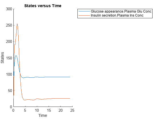
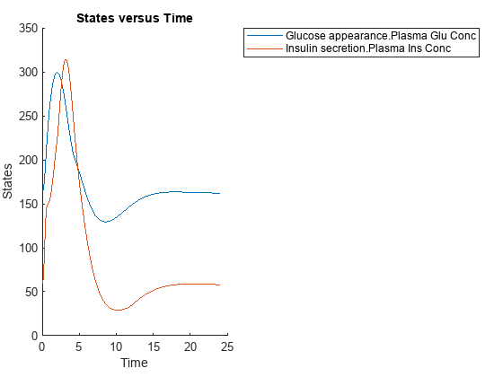
Simulate the glucose-insulin response for a normal subject for 24 hours.

sbioplot(normSim([],24,mealTable));

Figure contains an axes object. The axes object with title States versus Time, xlabel Time, ylabel States contains 2 objects of type line. These objects represent Glucose appearance.Plasma Glu Conc, Insulin secretion.Plasma Ins Conc.

Simulate the glucose-insulin response for a diabetic subject for 24 hours.

sbioplot(diabSim([],24,mealTable));

Perform a Scan Using Variants

Suppose you want to perform a parameter scan using an array of variants that contain different initial conditions for different insulin impairments. For example, the model m1 has variants that correspond to the low insulin sensitivity and high insulin sensitivity. You can simulate the model for both conditions via a single call to the SimFunction object.

Select the variants to scan.

varToScan = sbioselect(m1,'Name',...
                    {'Low insulin sensitivity','High insulin sensitivity'});

Check which model parameters are being stored in each variant.

varToScan(1)

ans = 
   SimBiology Variant - Low insulin sensitivity (inactive)

   ContentIndex:     Type:        Name:             Property:           Value:
   1                 parameter    Vmx               Value               .0235
   2                 parameter    kp3               Value               .0045

varToScan(2)

ans = 
   SimBiology Variant - High insulin sensitivity (inactive)

   ContentIndex:     Type:        Name:             Property:           Value:
   1                 parameter    Vmx               Value               .094
   2                 parameter    kp3               Value               .018

Both variants store alternate values for Vmx and kp3 parameters. You need to specify them as input parameters when you create a SimFunction object.

Create a SimFunction object to scan the variants.

variantScan = createSimFunction(m1,{'Vmx','kp3'},...
          {'[Plasma Glu Conc]','[Plasma Ins Conc]'},'Dose');

Simulate the model and plot the results. Run 1 include simulation results for the low insulin sensitivity and Run 2 for the high insulin sensitivity.

sbioplot(variantScan(varToScan,24,mealTable));

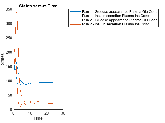
Figure contains an axes object. The axes object with title States versus Time, xlabel Time, ylabel States contains 4 objects of type line. These objects represent Run 1 - Glucose appearance.Plasma Glu Conc, Run 1 - Insulin secretion.Plasma Ins Conc, Run 2 - Glucose appearance.Plasma Glu Conc, Run 2 - Insulin secretion.Plasma Ins Conc.

Low insulin sensitivity lead to increased and prolonged plasma glucose concentration.

Restore warning settings.

warning(warnSettings);

Input Arguments

collapse all

`model` — SimBiology model
`SimBiology.Model` object

SimBiology model, specified as a SimBiology model object.

The function uses the same configset settings by making a copy of the Configset object of the model object. However, the function ignores the following configset settings: StatesToLog, OutputTimes, StopTime, and SensitivityAnalysisOptions because these settings are provided by other inputs to the function.

`params` — Inputs of SimFunction `F`
character vector | string scalar | string vector | cell array of character vectors | `{}` | `SimBiology.Scenarios` object

Inputs of SimFunction F, specified as a character vector, string scalar, string vector, cell array of character vectors, empty cell array {}, or SimBiology.Scenarios object. The character vectors represent the names of model quantities (species, compartments, or parameters) that define the inputs of F. Use an empty cell array {} or empty Scenarios object SimBiology.Scenarios.empty() to create a SimFunction object that has no parameters.

To unambiguously name a model quantity, use the qualified name, which includes the name of the compartment. To name a reaction-scoped parameter, use the reaction name to qualify the parameter. If the name is not a valid MATLAB^® variable name, surround it by square brackets such as [reaction 1].[parameter 1].

`observables` — Outputs of SimFunction `F`
character vector | string scalar | string vector | cell array of character vectors

Outputs of SimFunction F, specified as a character vector, string scalar, string vector, or cell array of character vectors. The character vectors represent the names of model quantities (species, compartments, or parameters) or observable objects that define the outputs of F.

`dosed` — Dosed species or dose objects
character vector | string scalar | string vector | cell array of character vectors | vector of dose objects | `[]`

Dosed species or dose objects, specified as a character vector, string scalar, string vector, cell array of character vectors, vector of dose objects, or empty array [].

If it is [], no species are dosed during simulation unless you specify a Scenarios object that has doses defined in its entries.

If it is a cell array of character vectors, it must be 1-by-N array, where N is the number of dosed species names. You can use duplicate species names if you plan to use multiple doses for the same species when you run the SimFunction F. Using only dosed species names contains no information on the dose properties. If you have a dose object that contains parameterized properties such as Amount, use the dose object as input instead of just species names to transfer such parameter information to the created SimFunction F.

If it is a vector of dose objects, it must be 1-by-N vector, where N is the number of dose objects. If dose objects have properties with nondefault numeric values, these values are ignored and a warning is issued. Only TargetName, DurationParameterName, LagParameterName, and parameterized properties are used to create the SimFunction object F, that is, to define the Dosed property of F. For details on how the Dosed property table is populated, see Dosed.

The dosing information that you specify during the creation of the SimFunction object must be consistent with the dosing information you specify during the execution of the object. In other words, the number of elements in the Dosed property of SimFunction F must equal to the combined number of doses in the input Scenarios object in phi and doses in the input argument u when you execute the object.

`variants` — Alternate model values
variant object | vector of variant objects

Alternate model values, specified as a variant or vector of variant objects. These values are applied as the model baseline values when the SimFunction object is created. If there are multiple variants referring to the same model element, the last occurrence is used.

Name-Value Arguments

Specify optional pairs of arguments as Name1=Value1,...,NameN=ValueN, where Name is the argument name and Value is the corresponding value. Name-value arguments must appear after other arguments, but the order of the pairs does not matter.

Example: F = createSimFunction(model,params,observables,dosed,UseParallel=true) specifies to execute the SimFunction F in parallel.

`UseParallel` — Flag to execute SimFunction `F` in parallel
`false` (default) | `true`

Flag to execute SimFunction F in parallel, specified as true or false. If true and Parallel Computing Toolbox™ is available, the SimFunction F is executed in parallel.

`AutoAccelerate` — Flag to accelerate model on first evaluation of `SimFunction`
`true` (default) | `false`

Flag to accelerate the model on the first evaluation of the SimFunction object, specified as true or false.

Set the value to false if you have a model that is fast to simulate because the acceleration of the model could take longer than the actual simulation of the model.

`SensitivityOutputs` — Sensitivity output factors
`{}` (default) | cell array of character vectors | `'all'`

Sensitivity output factors, specified as a cell array of character vectors. The character vectors are the names of model quantities (species and parameters) for which you want to compute the sensitivities. The default is {} meaning there is no output factors. Output factors are the numerators of time-dependent derivatives explained in Sensitivity Analysis in SimBiology.

Use the keyword 'all' or "all" to specify all model quantities as sensitivity outputs. However, {'all'} means a model quantity named all in the model. ["all","x"] sets the sensitivity input factors or output factors to the species named all and x.

You must specify both SensitivityOutputs and SensitivityInputs name-value arguments for sensitivity calculations.

Example: SensitivityOutputs='all'

`SensitivityInputs` — Sensitivity input factors
`{}` (default) | cell array of character vectors | `'all'`

Sensitivity input factors, specified as a cell array of character vectors. The character vectors are the names of model quantities (species, compartments, and parameters) with respect to which you want to compute the sensitivities. The default is {} meaning no input factors. Input factors are the denominators of time-dependent derivatives explained in Sensitivity Analysis in SimBiology.

You must specify both SensitivityOutputs and SensitivityInputs name-value arguments for sensitivity calculations.

Example: SensitivityInputs={'Reaction1.c1','Reaction1.c2'},

`SensitivityNormalization` — Normalization for calculated sensitivities
`'None'` (default) | `'Half` | `'Full'`

Normalization for calculated sensitivities, specified as one of the following: 'None', 'Half', or 'Full'.

'None' — No normalization (default)
'Half' — Normalization relative to the numerator only
'Full' — Full dedimensionalization

For details, see Normalization.

Example: SensitivityNormalization='Full'

Output Arguments

collapse all

`F` — SimFunction
`SimFunction` object | `SimFunctionSensitivity` object

SimFunction, returned as a SimFunction object or SimFunctionSensitivity object.

F is a SimFunctionSensitivity object if you specify non-empty 'SensitivityOutputs' and 'SensitivityInputs' name-value pair arguments.

References

[1] Gillespie, D.T. (1977). Exact Stochastic Simulation of Coupled Chemical Reactions. The Journal of Physical Chemistry. 81(25), 2340–2361.

Extended Capabilities

Automatic Parallel Support
Accelerate code by automatically running computation in parallel using Parallel Computing Toolbox™.

To run in parallel, set 'UseParallel' to true.

For more information, see the 'UseParallel' name-value pair argument.

Version History

Introduced in R2014a

createSimFunction

Syntax

Description

Examples

Create a SimFunction Object

Create a SimFunction Object with Dosing Information

Scan Parameters of the Lotka-Volterra Model

Calculate Local Sensitivities Using `SimFunctionSensitivity` Object

Simulate Model of Glucose-Insulin Response with Different Initial Conditions

Input Arguments

`model` — SimBiology model
`SimBiology.Model` object

`params` — Inputs of SimFunction `F`
character vector | string scalar | string vector | cell array of character vectors | `{}` | `SimBiology.Scenarios` object

`observables` — Outputs of SimFunction `F`
character vector | string scalar | string vector | cell array of character vectors

`dosed` — Dosed species or dose objects
character vector | string scalar | string vector | cell array of character vectors | vector of dose objects | `[]`

`variants` — Alternate model values
variant object | vector of variant objects

Name-Value Arguments

`UseParallel` — Flag to execute SimFunction `F` in parallel
`false` (default) | `true`

`AutoAccelerate` — Flag to accelerate model on first evaluation of `SimFunction`
`true` (default) | `false`

`SensitivityOutputs` — Sensitivity output factors
`{}` (default) | cell array of character vectors | `'all'`

`SensitivityInputs` — Sensitivity input factors
`{}` (default) | cell array of character vectors | `'all'`

`SensitivityNormalization` — Normalization for calculated sensitivities
`'None'` (default) | `'Half` | `'Full'`

Output Arguments

`F` — SimFunction
`SimFunction` object | `SimFunctionSensitivity` object

References

Extended Capabilities

Automatic Parallel Support
Accelerate code by automatically running computation in parallel using Parallel Computing Toolbox™.

Version History

See Also

Topics

createSimFunction

Syntax

Description

Examples

Create a SimFunction Object

Create a SimFunction Object with Dosing Information

Scan Parameters of the Lotka-Volterra Model

Calculate Local Sensitivities Using SimFunctionSensitivity Object

Simulate Model of Glucose-Insulin Response with Different Initial Conditions

Input Arguments

model — SimBiology model SimBiology.Model object

params — Inputs of SimFunction F character vector | string scalar | string vector | cell array of character vectors | {} | SimBiology.Scenarios object

observables — Outputs of SimFunction F character vector | string scalar | string vector | cell array of character vectors

dosed — Dosed species or dose objects character vector | string scalar | string vector | cell array of character vectors | vector of dose objects | []

variants — Alternate model values variant object | vector of variant objects

Name-Value Arguments

UseParallel — Flag to execute SimFunction F in parallel false (default) | true

AutoAccelerate — Flag to accelerate model on first evaluation of SimFunction true (default) | false

SensitivityOutputs — Sensitivity output factors {} (default) | cell array of character vectors | 'all'

SensitivityInputs — Sensitivity input factors {} (default) | cell array of character vectors | 'all'

SensitivityNormalization — Normalization for calculated sensitivities 'None' (default) | 'Half | 'Full'

Output Arguments

F — SimFunction SimFunction object | SimFunctionSensitivity object

References

Extended Capabilities

Automatic Parallel Support Accelerate code by automatically running computation in parallel using Parallel Computing Toolbox™.

Version History

See Also

Topics

Calculate Local Sensitivities Using `SimFunctionSensitivity` Object

`model` — SimBiology model
`SimBiology.Model` object

`params` — Inputs of SimFunction `F`
character vector | string scalar | string vector | cell array of character vectors | `{}` | `SimBiology.Scenarios` object

`observables` — Outputs of SimFunction `F`
character vector | string scalar | string vector | cell array of character vectors

`dosed` — Dosed species or dose objects
character vector | string scalar | string vector | cell array of character vectors | vector of dose objects | `[]`

`variants` — Alternate model values
variant object | vector of variant objects

`UseParallel` — Flag to execute SimFunction `F` in parallel
`false` (default) | `true`

`AutoAccelerate` — Flag to accelerate model on first evaluation of `SimFunction`
`true` (default) | `false`

`SensitivityOutputs` — Sensitivity output factors
`{}` (default) | cell array of character vectors | `'all'`

`SensitivityInputs` — Sensitivity input factors
`{}` (default) | cell array of character vectors | `'all'`

`SensitivityNormalization` — Normalization for calculated sensitivities
`'None'` (default) | `'Half` | `'Full'`

`F` — SimFunction
`SimFunction` object | `SimFunctionSensitivity` object

Automatic Parallel Support
Accelerate code by automatically running computation in parallel using Parallel Computing Toolbox™.