Heat Transfer in Insulated Oil Pipeline
Oil Pipelines
Temperature plays an important role in oil pipeline design. Below the so-called cloud point, paraffin waxes precipitate from crude oil and start to accumulate along the pipe wall interior. The waxy deposits restrict oil flow, increasing the power requirements of the pipeline. At still-lower temperatures—below the pour point of oil—these crystals become so numerous that, if allowed to quiesce, oil becomes semisolid.
In cold climates, conductive heat losses through the pipe wall can be significant. To keep oil in its favorable temperature range, pipelines include some temperature control measures. Heating stations placed at intervals along the pipeline help to warm the oil. An insulant liner covering the pipe wall interior helps to retard the cooling rate of the oil.
Viscous dissipation provides an additional heat source. As adjacent parcels of oil flow against each other, they experience energy losses that appear in the form of heat. The warming effect is small, but sufficient to at least partially offset the conductive heat losses that occur through the insulant liner.
At a certain insulation thickness, viscous dissipation exactly balances the conductive heat loss. Oil stays at its ideal temperature throughout the pipeline length and the need for heating stations is reduced. From a design standpoint, this insulation thickness is optimal.
In this example, you simulate an insulated oil pipeline segment. You then run an optimization script to determine the optimal insulation thickness. This example is based on the Optimal Pipeline Geometry for Heated Oil Transportation example model.
Modeling Considerations
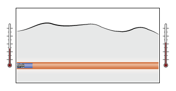
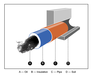
The physical system in this example is an oil pipeline segment. Insulation lines the pipe wall interior, while soil covers the pipe wall exterior, retarding conductive heat loss. The simplifying assumption is made that the physical system is symmetric about the pipe center line.
Flow through the pipeline segment is assumed fully developed: the velocity profile of the flowing oil remains constant along the pipeline length. In addition, oil is assumed Newtonian and compressible: shear stress is proportional to the shear strain, and mass density varies with both temperature and pressure.
Oil enters the pipeline segment at a fixed temperature, TUpstream, with a fixed mass flow rate, Vdot * rho0, where:
Vdot is the volumetric flow rate of oil through the pipe.
rho0 is the mass density of oil entering the pipeline segment.
Inside the pipeline segment, viscous dissipation heats the flowing oil, while thermal conduction through the pipe wall cools it. The balance between the two processes governs the temperature of oil exiting the pipeline segment.
The amount of heat gained through viscous dissipation depends partly on oil viscosity and mass flow rate. The greater these quantities are, the greater the viscous heat gain is, and the warmer the oil tends to get. The amount of heat lost via thermal conduction depends partly on the thermal resistances of the insulation, pipe wall, and soil layer. The smaller the thermal resistances are, the greater the conductive heat loss is, and the cooler the oil tends to get.
Using an electrical circuit analogy, the combined thermal resistance of three material layers arranged in series equals the sum of the individual thermal resistances:
Rcombined = Rwall + Rins. + Rsoil
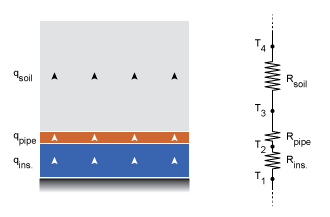
Assuming the pipe wall is thin and its material is a good thermal conductor, you can safely ignore the thermal resistance of the pipe wall. The combined thermal resistance is then simply the sum of the insulation and soil contributions, Rins. and Rsoil.
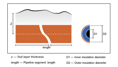
The thermal resistance of the insulation layer is directly proportional to its thickness, (D2-D1)/2, and inversely proportional to its thermal conductivity, kInsulant. Likewise, the thermal resistance of the soil layer is directly proportional to its thickness, z, and inversely proportional to its thermal conductivity, kSoil.
The figure shows the relevant dimensions of the pipeline segment. Variable names match those specified in the model. The inner insulation diameter, D1, is also the hydraulic diameter of the pipeline segment.
Explore Model
The Optimal Pipeline Geometry for Heated Oil Transportation example model represents an insulated oil pipeline segment buried underground. To open this model, at the MATLAB® command prompt, enter:
openExample('simscape/OptimalPipelineGeometryForHeatedOilTransportationExample')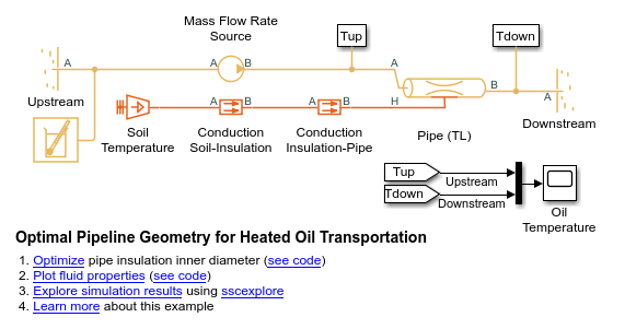
The Pipe (TL) block represents the physical system in this example, that is, the oil pipeline segment. Port A represents its inlet and port B its outlet. Port H represents thermal conduction through the pipe wall. The block accounts for viscous heating.
The Flow Rate Source (TL) block provides the flow rate through the pipe. The Upstream block acts as a temperature source for the pipe inlet, while the Downstream block acts as a temperature sink at the pipe outlet.
The Conduction Insulation-Pipe and Conduction Soil-Insulation blocks represent thermal conduction through insulant and soil layers, respectively. These blocks appear in the Simscape™ Thermal library as Conductive Heat Transfer. The Soil Temperature (Temperature Source) block provides the temperature boundary condition at the soil surface.
The Thermal Liquid Settings (TL) block provides the physical properties of the oil, expressed as two-dimensional lookup tables containing the temperature and pressure dependence of the properties. The table summarizes these blocks.
| Block | Description |
|---|---|
| Pipe (TL) | Pipeline segment |
| Conduction Insulation-Pipe | Insulant thermal conduction |
| Conduction Soil-Insulation | Soil thermal conduction |
| Soil Temperature | Soil temperature |
| Upstream | Pipe inlet temperature sink |
| Downstream | Pipe outlet temperature sink |
| Flow Rate Source (TL) | Oil mass flow rate |
| Thermal Liquid Settings (TL) | Oil thermodynamic properties |
Run Simulation
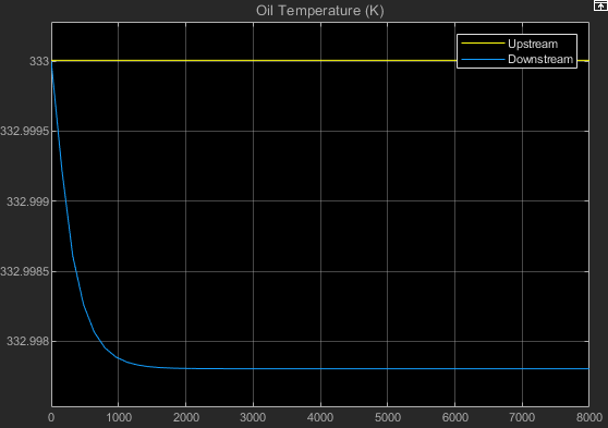
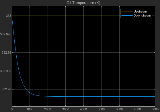
To analyze the performance of the oil pipeline segment, simulate the model. The Oil Temperature scope plots the upstream and downstream oil temperatures. Open this scope. The insulation thickness is near its optimal value, resulting in only a small temperature change over a 1000 meter length. At a rate of ~0.020 K/km, oil temperature changes approximately 2 K over a 100 kilometer length.
Plot Physical Properties Using Data Logging
As an alternative to using sensors and scopes, you can use Simscape data logging to view how the physical properties of oil and other system variables change during simulation.
Select the Pipe (TL) block.
On the Simscape Block tab at the top of the model window, under Review Results, click Results Explorer.
In the left pane of the Simscape Results Explorer window, expand the
Pipe
                                (TL)
node, which contains logged data for the Pipe (TL) block. Then expand theAandBnodes, which correspond to the A and B ports of the block.Select variable
Tunder nodeA, which is the upstream temperature of the pipe, to display its plot in the right pane of the Simscape Results Explorer window. To plot multiple variables at once, press theCtrlkey and select variableTunder nodeB, which is the downstream temperature of the pipe.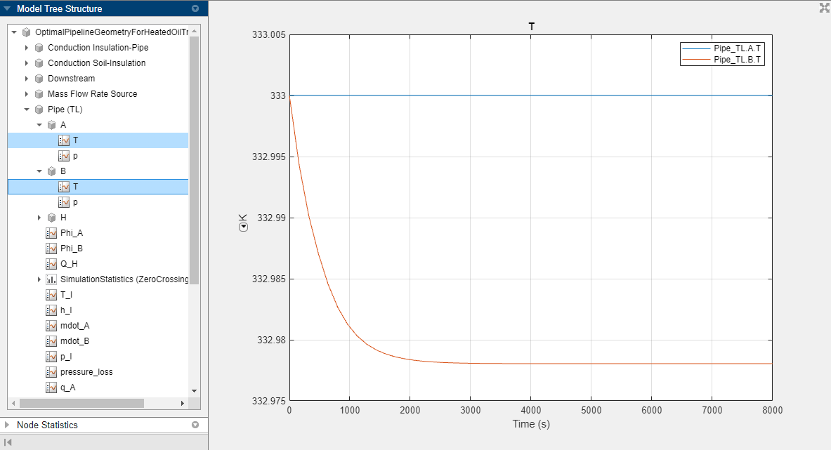
As expected, the plots in the right pane of the Simscape Results Explorer window are equivalent to the Oil Temperature scope results.
You can also use the Simscape Results Explorer to plot other physical properties of the oil as a function of simulation time. For example,
rho_Iis the oil density.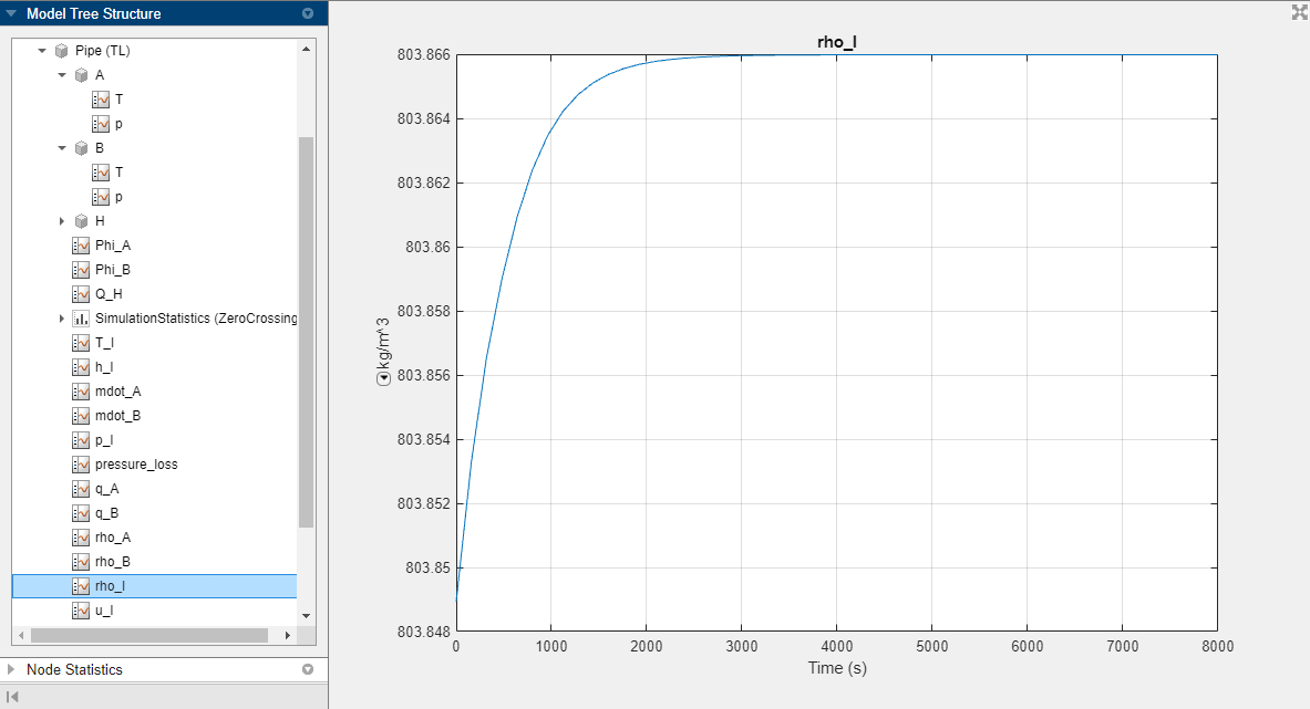
Note
For more information about Simscape logging, see About Simscape Data Logging.
Simulate Effects of Changing Insulation Diameter
Experiment with different values for the insulation inner diameter. By varying this parameter, you offset the balance between viscous dissipation, which heats the oil, and thermal conduction, which cools the oil.
Open Model Explorer.
In the Model Hierarchy pane, select Base Workspace.
In the Contents pane, click the value of parameter D1.
Enter
0.20.
By reducing the inner diameter of the insulation layer to 0.20, you increase the insulation thickness, slowing down heat loss through the pipe wall via thermal conduction. Run the simulation. Then, open the Oil Temperature scope and autoscale to view full plot.
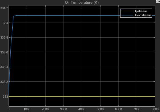
The new plot shows an oil temperature at the pipe outlet (top curve) that significantly exceeds the temperature at the pipe inlet (bottom line). Viscous dissipation now dominates the thermal energy balance in the pipeline segment. The new insulation thickness poses a design problem: in a long pipeline, a 1.1 K/km heating rate can raise the oil temperature substantially at the receiving end of the pipeline.
Try increasing the inner diameter of the insulation layer, D1, to 0.55. By increasing this value, you decrease the insulation thickness, accelerating heat loss through the pipe wall via thermal conduction. Then, run the simulation. Open the Oil Temperature scope and autoscale to view the full plot.
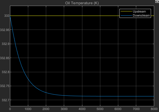
The resulting plot shows that the oil temperature at the pipe outlet is now significantly lower than that at the pipe inlet. Thermal conduction clearly dominates the thermal energy balance in the pipeline segment. This insulation thickness also poses a design issue: at a rate of 0.25K/km, oil flowing through a long pipeline will cool down substantially.
Run Optimization Script
The model provides an optimization script that you can run to determine the optimal inner diameter of the pipe insulation, D1. The script iterates the model simulation at different D1 values, plotting the rates of viscous warming and conductive cooling against each other. The intersection point between the two curves identifies the optimal insulation thickness for the model:
In the model window, click Optimize to run the optimization script for the pipe insulation inner diameter.
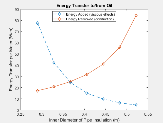
In the plot that opens, visually determine the horizontal-axis value for the intersection point between the two curves.
The optimal inner diameter of the insulation layer is 0.37 m. Update parameter D1 to this value:
Open Model Explorer.
In the Model Hierarchy pane, click Base Workspace.
In the Contents pane, click the value of D1.
Enter
0.37.
Now, run the simulation. Open the Oil Temperature scope and autoscale to view the full plot. The temperature difference between the inlet and the outlet is negligible.