Analyze Results Using Simulation Manager

The Simulation Manager allows you to monitor multiple simulations, in serial or in parallel, and their progress. You can view the details of every run, such as parameters, elapsed time, and diagnostics. The Simulation Manager provides the option to analyze and compare your logged signal results in the Simulation Data Inspector. Through Simulation Manager, you can select a run and apply its values to the model. Simulation Manager opens when you run a parsim or a sim command with ShowSimulationManager argument set to on. For more information, see Simulation Manager.

The dimensions of the tank have an impact on the total cost of production of the product. For this example, we observe the behavior of TotalCost for different values of the width and the height. By analyzing the behavior of the parameters, we find the combination of A and h that results in lowest TotalCost. To solve this design problem, we run multiple simulations (in parallel or in serial) with different values of the parameters A and h.

This example shows how you can use the Simulation Manager to analyze the simulations and solve a design problem using a model of a continually stirred tank reactor. The reactors are specialized tanks that are used to mix various chemicals or compounds to create a product. The important variables used in this model are:

Variable A, which represents the cross-sectional area of the tank (width).
Variable h, which represents the height.
Variable TotalCost, which represents the cost, in dollars, to produce a tankful of product.

Simulation Manager enables you to analyze the simulations as they are running. When the simulations are in progress, you can visualize the simulation data of the model by plotting the simulation outputs against the input parameters. Visualizing trend of the simulations as they are happening allows you to learn about the design space of the simulations and evaluate whether the simulations are running as required. You can stop the simulations if the progress is not as desired thus saving time.

Open Simulation Manager

In this example, use a set of sweep parameters provided to the model through Simulink.SimulationInput objects and then use the parsim command to run the simulations in parallel.

Open the model.

openExample('simulink/OpenTheModelToUseWithSimulationManagerExample');
open_system('simManagerCSTR');

Create a PostSimFcn function as follows in a MATLAB script to call later in the parameter sweep. Name the file calculateCost.m. The PostSimFcn function calculates TotalCost from the variables A and h, and its calculation can vary depending on the application.

function costOutput = calculateCost(out)

    costOutput.yout = out.yout;
    
    coolantOutput = out.yout.get('Coolant').Values.Data;
    costCoolant = abs(mean(coolantOutput - 294))/30;
    costOutput.costFromCoolant = costCoolant;
    
    concentrationOutput = out.yout.get('Residual Concentration').Values.Data;
    costConcentration = 10*std(concentrationOutput - 2);
    costOutput.costFromConcentration = costConcentration;
    
    costOutput.TotalCost = costCoolant + costConcentration;
    
end

Create a sample of values for parameter sweep.

rangeA = [0.1, 5];
rangeH = [0.1, 5];

rng default;

numSamples = 60;
allAValues = rangeA(1) + (rangeA(2) - rangeA(1)).*rand(numSamples, 1);
allhValues = rangeH(1) + (rangeH(2) - rangeH(1)).*rand(numSamples, 1);

Create an array of Simulink.SimulationInput objects. For this example, the TotalCost is calculated and returned using the PostSimFcn.

in(1:numSamples) = Simulink.SimulationInput('simManagerCSTR');
in = in.setPostSimFcn(@(out)calculateCost(out));

Run the simulations in parallel and open the Simulation Manager.


for k = 1:numSamples
    in(k) = in(k).setVariable('A', allAValues(k), 'Workspace', 'simManagerCSTR');
    in(k) = in(k).setVariable('h', allhValues(k), 'Workspace', 'simManagerCSTR');
end

out = parsim(in, 'ShowSimulationManager', 'on');

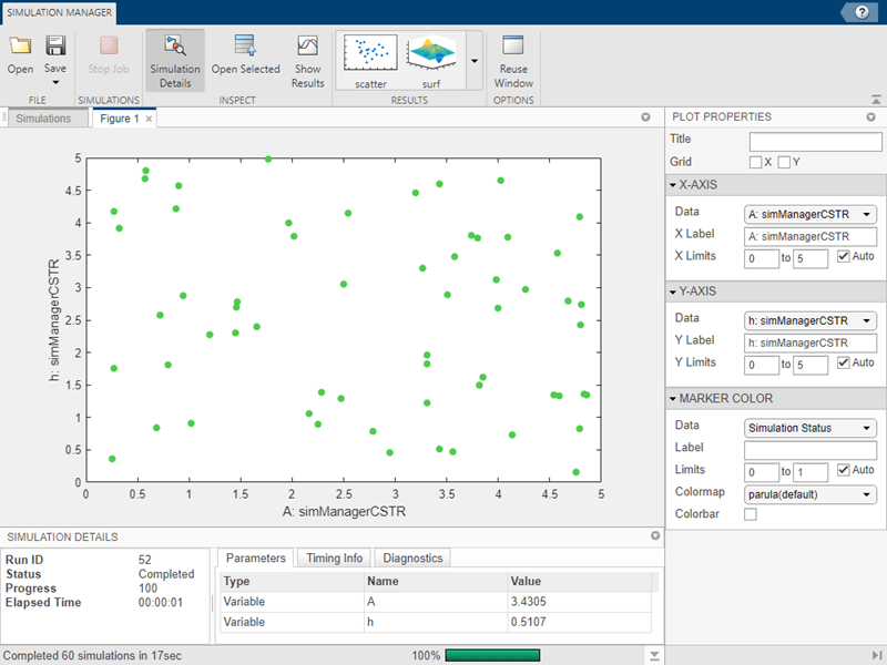
The default view in the Simulation Manager shows a scatter plot with two parameters on its X and Y axes. In this case, the variable A is on the X-axis and variable h is on the Y-axis. When the simulations are running you can see dots appear on the plot, color coded according to the simulation status. Completed simulations are marked in green, in-progress simulations are blue, and simulations with errors are red.

The Plot Properties panel on the right enables you to edit and configure the data that plot shows. By selecting grid for X and Y axes, the plot appears with grid lines.

If a particular parameter is a time-series, the Simulation Manager plots only the last value of the time series.

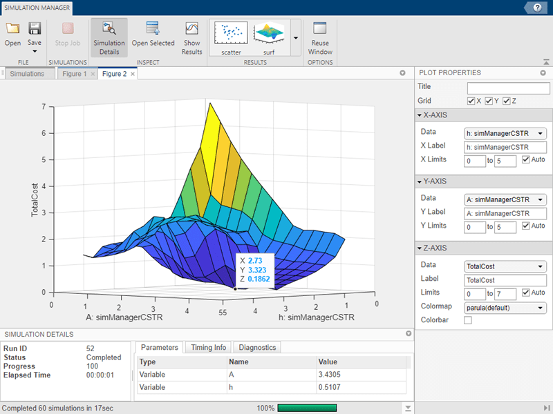
With the Simulation Manager, you can visualize the above data in a surf plot. Click the surf plot in the Results section of the toolstrip.

Add and Configure Plots

The Results section of the Simulation Manager allows you to add multiple plots and configure them. To add a plot, click the type of the plot in the Results section. For this example, click the surf plot in Results section of the Simulation Manager toolstrip. Using the plot properties, change the parameters to display on the plots. You can change properties such as the plot labels, axes labels and you can add a colormap to denote the third parameter. You can also change the value limits of the colormap.

With the second plot and the first plot together, you can determine the value of the variables A and h, that gives the best TotalCost.

For the Z-axis of the surf plot, change the Data to TotalCost. By observing the surf plot, you can find the lowest point of TotalCost. Clicking the lowest point shows the values for X-axis and Y-axis, which is h and A, respectively.

Save and Load Simulation Manager

Save the session information, which includes simulation data all the plot configurations. To save the session, click the Save button on the toolstrip. The session saves as a .mldatx file. To reopen the saved session, navigate to the location where the file is saved and double-click the .mldatx file.

The Simulation Manager allows you to reuse the plot configuration when you want to run similar simulations with different sets of values. To reuse the plot configuration, click the Reuse Window button on the toolstrip. Selecting the Reuse Window saves the plot configurations, such as labels, axis orientation, which parameters to display on which axis that you can reuse with the next simulation of the same model. When you use this functionality while running simulations for different models, the simulation errors out due to a limitation.