Attitude Control in the HL-20 Autopilot - MIMO Design
This is Part 4 of the example series on design and tuning of the flight control system for the HL-20 vehicle. This part shows how to tune a MIMO PI architecture for controlling the roll, pitch, and yaw of the vehicle.
Background
This example uses the HL-20 model adapted from NASA HL-20 Lifting Body Airframe (Aerospace Blockset); see Part 1 of the series (Trimming and Linearization of the HL-20 Airframe) for details. In Parts 2 and 3, we showed how to close the inner loops and tune the outer loops of a classic SISO architecture for the HL-20 autopilot; see Angular Rate Control in the HL-20 Autopilot and Attitude Control in the HL-20 Autopilot - SISO Design for details. In this example, we explore the benefits of switching to a MIMO architecture for the outer loops.

In this architecture, the three PI loops for pitch, alpha, beta are replaced by a 3-input, 3-output PI controller that blends the pitch, alpha, and beta measurements to calculate the inner-loop setpoints p_demand, q_demand, r_demand. Intuitively, this architecture should be more successful at reducing cross-couplings between axes. Note that the P and I gains are 3-by-3 matrices scheduled as a function of alpha and beta.
To get started, load the model, set CTYPE to 3 to select the MIMO variant of the Controller block, and reapply the steps of Part 2 for closing the inner loops (this part of the design is unchanged). Note that this creates and configures an slTuner interface ST0 for interacting with the Simulink® model.
load_system('csthl20_control')
CTYPE = 3;  % MIMO architecture
HL20recapPart2

ST0
slTuner tuning interface for "csthl20_control":

No tuned blocks. Use the addBlock command to add new blocks.
9 Analysis points:
--------------------------
Point 1: Signal "da;de;dr", located at 'Output Port 1' of csthl20_control/Flight Control System/Controller
Point 2: Signal "pqr", located at 'Output Port 2' of csthl20_control/HL20 Airframe
Point 3: 'Output Port 1' of csthl20_control/Flight Control System/Alpha_deg
Point 4: 'Output Port 1' of csthl20_control/Flight Control System/Beta_deg
Point 5: 'Output Port 1' of csthl20_control/Flight Control System/Phi_deg
Point 6: 'Output Port 1' of csthl20_control/Flight Control System/Controller/MIMO/Demands
Point 7: Signal "p_demand", located at 'Output Port 1' of csthl20_control/Flight Control System/Controller/MIMO/Roll-off1
Point 8: Signal "q_demand", located at 'Output Port 1' of csthl20_control/Flight Control System/Controller/MIMO/Roll-off2
Point 9: Signal "r_demand", located at 'Output Port 1' of csthl20_control/Flight Control System/Controller/MIMO/Roll-off3

No permanent openings. Use the addOpening command to add new permanent openings.
Properties with dot notation get/set access:
      Parameters         : []
      OperatingPoints    : [] (model initial condition will be used.)
      BlockSubstitutions : [3x1 struct]
      Options            : [1x1 linearize.SlTunerOptions]
      Ts                 : 0
Setup for Outer Loop Tuning
As in the SISO design (Attitude Control in the HL-20 Autopilot - SISO Design), the first step is to obtain a linearized model of the "plant" seen by the outer loops at each (alpha,beta) condition. To account for the fact that the inner-loop gains Kp,Kq,Kr vary with (alpha,beta), replace the "MIMO/Product" block by its linear equivalent, which is the diagonal gain matrix
Blk = 'csthl20_control/Flight Control System/Controller/MIMO/Product';
Subs = [zeros(3) append(ss(Kp),ss(Kq),ss(Kr))];
BlockSub4 = struct('Name',Blk,'Value',Subs);

ST0.BlockSubstitutions = [ST0.BlockSubstitutions ; BlockSub4];
The gain schedules "P" and "I" are initialized to the constant diagonal matrices diag([0.05, 0.05, -0.05]). Plot the angular responses for these initial settings.
T0 = getIOTransfer(ST0,'Demand',{'Phi_deg','Alpha_deg','Beta_deg'});
step(T0,6)

Tuning Goals
To tune the MIMO gain schedules we use the following three tuning goals:
A "Sensitivity" goal to specify the desired bandwidth (response time) and maximize decoupling at low frequency.
s = tf('s');
R1 = TuningGoal.Sensitivity({'Phi_deg','Alpha_deg','Beta_deg'},s);
R1.Focus = [1e-2 1];
R1.LoopScaling = 'off';

viewGoal(R1)

A "Gain" constraint on the closed-loop transfer from angular demands to angular responses. The gain profile is chosen to enforce adequate roll-off and limit overshoot (which is related to the hump near crossover).
MaxGain = 1.2 * (10/(s+10))^2;  % max gain profile
R2 = TuningGoal.Gain('Demands',{'Phi_deg','Alpha_deg','Beta_deg'},MaxGain);

viewGoal(R2)
A "Margins" goal to require gain margins of at least 7 dB and phase margins of at least 45 degrees (in the disk margin sense).
R3 = TuningGoal.Margins('da;de;dr',7,45);Gain Schedule Tuning
The gain schedules for the MIMO PI controller are specified by the "P" and "I" blocks in the MIMO architecture. Recall that these blocks output 3-by-3 matrices and implement the MIMO transfer function:
For illustration sake, we use a MATLAB Function block to implement the proportional gain schedule, and a Matrix Interpolation block to implement the integral gain schedule. The Matrix Interpolation block lives in the "Simulink Extras" library and is a lookup table where each table entry is a matrix.
To tune the P and I gain schedules, mark the corresponding blocks as tunable in the slTuner interface.
TunedBlocks = {'MIMO/P' , 'MIMO/I'};
ST0.addBlock(TunedBlocks)
Parameterize each tuned gain schedule as a polynomial surface in alpha and beta. Again we use a quadratic surface for the proportional gain and a multilinear surface for the integral gain.
% Grid of (alpha,beta) design points
alpha_vec = -10:5:25;	 % Alpha Range
beta_vec = -10:5:10;     % Beta Range
[alpha,beta] = ndgrid(alpha_vec,beta_vec);
SG = struct('alpha',alpha,'beta',beta);

% Proportional gain matrix
alphabetaBasis = polyBasis('canonical',2,2);
P0 = diag([0.05 0.05 -0.05]);  % initial (constant) value
PS = tunableSurface('P', P0, SG, alphabetaBasis);
ST0.setBlockParam('P',PS);

% Integral gain matrix
alphaBasis = @(alpha) alpha;
betaBasis = @(beta) abs(beta);
alphabetaBasis = ndBasis(alphaBasis,betaBasis);
I0 = diag([0.05 0.05 -0.05]);
IS = tunableSurface('I', I0, SG, alphabetaBasis);
ST0.setBlockParam('I',IS);
Finally, use systune to tune the 6 gain surfaces against the three tuning goals.
ST = systune(ST0,[R1 R2 R3]);
Final: Soft = 1.13, Hard = -Inf, Iterations = 115
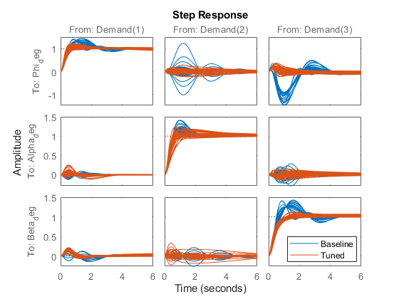
The final value of the objective function indicates that the tuning goals are nearly met (a tuning goal is satisfied when its "value" is less than one). Plot the closed-loop angular responses and compare with the baseline design.
T = getIOTransfer(ST,'Demand',{'Phi_deg','Alpha_deg','Beta_deg'});
step(T0,T,6)
legend('Baseline','Tuned','Location','SouthEast')
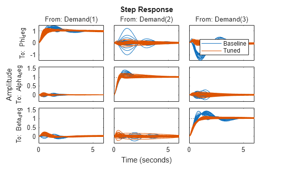
These responses show significant reductions in overshoot and cross-coupling when compared to the SISO design.
Validation
To further validate this design, push the tuned gain surfaces to the Simulink model.
writeBlockValue(ST);
For the Matrix Interpolation block "I", this samples the gain surface at the table breakpoints and updates the table data in the model workspace. For the MATLAB Function block "P", this generates MATLAB® code for the gain surface equations. You can see this code by double-clicking on the block.
Once you push the gains to Simulink, tuning of the MIMO architecture is complete and you can simulate its behavior during the landing approach.
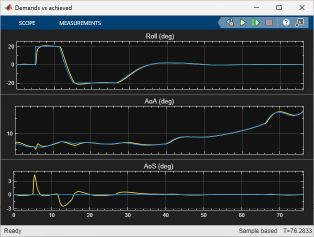
These responses are not very different from the SISO design (Attitude Control in the HL-20 Autopilot - SISO Design) due to the mild demands throughout the maneuver. The benefits of the MIMO design would be more visible in a more challenging maneuver.