Enforce Constraints for PID Controllers

This example uses:

This example shows how to enforce known constraints for a PID controller application using the Constraint Enforcement block.

Overview

For this example, the plant dynamics are described by the following equations [1].

$\begin{array}{l} {x_{}^{˙}}_{1} = - x_{1} + (x_{1}^{2} + 1) u_{1} \\ {x_{}^{˙}}_{2} = - x_{2} + (x_{2}^{2} + 1) u_{2} \end{array}$

The goal for the plant is to track desired trajectories, defined as:

$\begin{array}{l} θ_{}^{˙} = 0.1 π \\ {x_{}^{˙}}_{1 d} = - r \cos (θ) \\ {x_{}^{˙}}_{2 d} = r \sin (θ) \end{array}$

For an example that learns and applies an unknown constraint function for the same PID control application, see Learn and Apply Constraints for PID Controllers.

Configure model parameters and initial conditions.

r = 1.5;   % Radius for desired trajectory
Ts = 0.1;  % Sample time
Tf = 22;   % Duration
x0_1 = -r; % Initial condition for x1
x0_2 = 0;  % Initial condition for x2

Design PID Controllers

Before applying constraints, design PID controllers for tracking the reference trajectories. The trackingWithPIDs model contains two PID controllers with gains tuned using the PID Tuner app. For more information on tuning PID controllers in Simulink models, see Introduction to Model-Based PID Tuning in Simulink.

mdl = 'trackingWithPIDs';
open_system(mdl)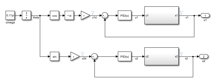

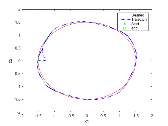
Simulate the PID controllers and plot their tracking performance.

% Simulate the model.
out = sim(mdl);

% Extract trajectories.
logData = out.logsout;
x1_traj = logData{3}.Values.Data;
x2_traj = logData{4}.Values.Data;
x1_des = logData{1}.Values.Data;
x2_des = logData{2}.Values.Data;

% Plot trajectories.
figure('Name','Tracking')
xlim([-2,2])
ylim([-2,2])
plot(x1_des,x2_des,'r')
xlabel('x1')
ylabel('x2')
hold on
plot(x1_traj,x2_traj,'b:','LineWidth',2)
hold on
plot(x1_traj(1),x2_traj(1),'g*')
hold on
plot(x1_traj(end),x2_traj(end),'go')
legend('Desired','Trajectory','Start','end')

Constraint Function

For this example, you apply known constraints to the application using the Constraint Enforcement block, which adjusts control actions to satisfy a constraint function.

In this example, the feasible region for the plant is given by ${x : x_{1} \leq 1, x_{x} \leq 1}$ . Therefore, the plant next-state condition $x_{k + 1} = [\begin{array}{c} x_{1} (k + 1) \\ x_{2} (k + 1) \end{array}]$ must satisfy $x_{k + 1} \leq [\begin{array}{c} 1 \\ 1 \end{array}]$ .

You can approximate the plant dynamics by the following equation.

$x_{k + 1} \approx [\begin{array}{c} (1 - T_{s}) & 0 \\ 0 & (1 - T_{s}) \end{array}] x_{k} + [\begin{array}{c} T_{s} (1 + x_{1}^{2} (k)) & 0 \\ 0 & T_{s} (1 + x_{2}^{2} (k)) \end{array}] u_{k}$

Applying the constraints to this equation produces the following constraint function.

$[\begin{array}{c} (1 - T_{s}) & 0 \\ 0 & (1 - T_{s}) \end{array}] x_{k} + [\begin{array}{c} T_{s} (1 + x_{1}^{2} (k)) & 0 \\ 0 & T_{s} (1 + x_{2}^{2} (k)) \end{array}] u_{k} \leq [\begin{array}{c} 1 \\ 1 \end{array}]$

The Constraint Enforcement block accepts constraints of the form $f_{x} + g_{x} u \leq c$ . For this application, the coefficients of this constraint function are as follows.

$f_{x} = [\begin{array}{c} (1 - T_{s}) & 0 \\ 0 & (1 - T_{s}) \end{array}] x_{k}, g_{x} = [\begin{array}{c} T_{s} (1 + x_{1}^{2} (k)) & 0 \\ 0 & T_{s} (1 + x_{2}^{2} (k)) \end{array}], c = [\begin{array}{c} 1 \\ 1 \end{array}]$

Simulate PID Controller with Constraint Enforcement

The trackingWithConstraintPID model contains the PID controllers, the plant dynamics and the constraint implementation.

mdl = 'trackingWithKnownConstraintPID';
open_system(mdl)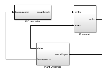

To view the constraint implementation, open the Constraint subsystem. Here, the model implements the known constraint function using a MATLAB Function block, and the Constraint Enforcement block enforces the constraint function.

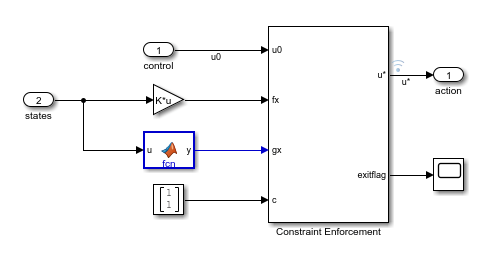
Run the model and plot the simulation results. The plot shows that the plant states are less than one.

% Simulate the model.
out = sim(mdl);

% Extract trajectories.
logData = out.logsout;
x1_traj = zeros(size(out.tout));
x2_traj = zeros(size(out.tout));
for ct = 1:size(out.tout,1)
    x1_traj(ct) = logData{4}.Values.Data(:,:,ct);
    x2_traj(ct) = logData{5}.Values.Data(:,:,ct);
end

x1_des = logData{2}.Values.Data;
x2_des = logData{3}.Values.Data;

% Plot trajectories.
figure('Name','Tracking with Constraint');
plot(x1_des,x2_des,'r')
xlabel('x1')
ylabel('x2')
hold on
plot(x1_traj,x2_traj,'b:','LineWidth',2)
hold on
plot(x1_traj(1),x2_traj(1),'g*')
hold on
plot(x1_traj(end),x2_traj(end),'go')
legend('Desired','Trajectory','Start','End','Location','best')

The Constraint Enforcement block successfully constrains the control actions such that the plant states remain less than one.

bdclose('trackingWithPIDs')
bdclose('trackingWithKnownConstraintPID')

References

[1] Robey, Alexander, Haimin Hu, Lars Lindemann, Hanwen Zhang, Dimos V. Dimarogonas, Stephen Tu, and Nikolai Matni. "Learning Control Barrier Functions from Expert Demonstrations." Preprint, submitted April 7, 2020. https://arxiv.org/abs/2004.03315