Enforce Passivity Constraints for Quadruple-Tank System

Overview

You can write the dynamics for a quadruple tank system as follows [1].

Here, the vector $\mathit{x}$ denotes the heights of the four tanks and the vector $\mathit{u}$ denotes the flows of the two pumps. The dynamics are implemented in the script stateFcnQuadrupleTank.m.

The control objective is to select the flow of the pumps $\mathit{u}$ such that $\left(\mathit{x},\mathit{u}\right)$ moves towards the equilibrium $\left({\mathit{x}}_{\mathit{s}},{\mathit{u}}_{\mathit{s}}\right)$.

Specify the initial conditions of the states.

x0 = [25;16;20;21];

Specify the equilibrium point for the quadruple-tank model.

xs = [28.1459,17.8230,18.3991,25.1192]';
us = [37,38]';

Design PID Controllers

Before applying constraints, design PID controllers for the quadruple-tank model. The passivityTank model contains two PID controllers. For information on tuning PID controllers in Simulink® models, see Introduction to Model-Based PID Tuning in Simulink.

Disable the passivity constraint enforcement and open the model.

constrained = 0;
mdl = 'passivityTank';
open_system(mdl)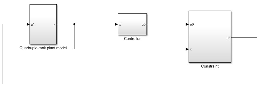

Simulate the PID controllers and plot the performance.

% Simulate the model.
out = sim(mdl);
% Extract trajectories.
logsout = out.logsout;
% Plot trajectories of state error.
e = logsout.getElement('states_error');       
e_vector = e.Values.Data(:,:)';
plot(e.Values.time,e_vector)
ylim([-6 6])
grid on
legend('e1','e2','e3','e4','location','NorthEast')
title('State Error')

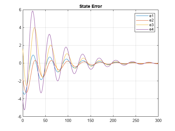
The errors go to zero and the closed loop system is stable.

Passivity Constraint

To define the passivity constraint, first define the state error vector:

$$\mathit{e}=\mathit{x}-{\mathit{x}}_{\mathit{s}}$$.

Define the storage function as $\mathit{V}=\frac{1}{2}({\mathit{e}}_3^2+{\mathit{e}}_4^2)$ and take the derivative of $\mathit{V}$ to obtain the following relationship [1].

This means that, the system is passive from ${\mathit{u}}_{\mathit{p}}=\left[{\mathit{u}}_1;{\mathit{u}}_2\right]-{\mathit{u}}_{\mathit{s}}$ to ${\mathit{y}}_{\mathit{p}}=\left[{\mathit{e}}_4;{\mathit{e}}_3\right]$.

The Passivity Enforcement block accepts passivity constraint in the forms ${\mathit{u}}_{\mathit{p}}={\mathit{f}}_{\mathit{p}}\left(\mathit{x}\right)+{\mathit{g}}_{\mathit{p}}\left(\mathit{x}\right)\mathit{u}$ and ${\mathit{y}}_{\mathit{p}}={\mathit{h}}_{\mathit{p}}\left(\mathit{x}\right)$. In this application,

${\mathit{f}}_{\mathit{p}}\left(\mathit{x}\right)=-{\mathit{u}}_{\mathit{s}}$, ${\mathit{g}}_{\mathit{p}}\left(\mathit{x}\right)=\left[\begin{array}{cc}1& 0\\ 0& 1\end{array}\right]$, and ${\mathit{h}}_{\mathit{p}}\left(\mathit{x}\right)=\left[\begin{array}{c}{\mathit{x}}_4-{\mathit{x}}_{\mathit{s},4}\\ {\mathit{x}}_3-{\mathit{x}}_{\mathit{s},3}\end{array}\right]$.

Simulate Controller with Passivity Constraint

To view the constraint implementation, open the Constraint > Constrained subsystem.

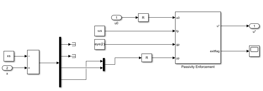
Enable the passivity constraint enforcement.

constrained = 1;

Run the model and plot the simulation results.

% Simulate the model.
out = sim(mdl);

% Extract trajectories.
logsout = out.logsout;

% Plot trajectories of state error.
e = logsout.getElement('states_error');       
e_vector = e.Values.Data(:,:)';
plot(e.Values.time,e_vector)
ylim([-6 6])
grid on
legend('e1','e2','e3','e4','location','NorthEast')
title('State Error')

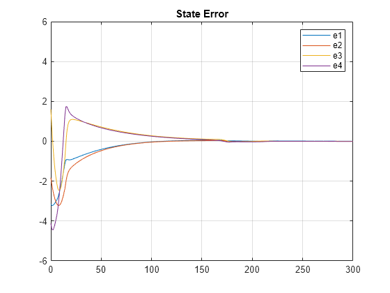
The errors go to zero and the closed loop system is stable. When you enforce passivity constraint, the errors have smaller magnitudes and smoother transient behavior.

% Plot trajectories of control inputs
u = logsout.getElement('u*');       
u_vector = u.Values.Data(:,:)';
plot(u.Values.time,u_vector)
grid on
legend('u1','u2','location','NorthEast')
title('Control Input')

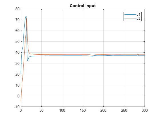
The control inputs also converge to the specified equilibrium.

Close the model.

bdclose(mdl)

References

[1] Raff, Tobias, Christian Ebenbauer, and Frank Allgöwer. “Nonlinear Model Predictive Control: A Passivity-Based Approach.” In Assessment and Future Directions of Nonlinear Model Predictive Control, edited by Rolf Findeisen, Frank Allgöwer, and Lorenz T. Biegler, 358:151-162. Berlin, Heidelberg: Springer Berlin Heidelberg, 2007. https://doi.org/10.1007/978-3-540-72699-9_12.