Model Computational Delay and Sampling Effects

Simulate Discrete and Continuous Controllers

In the following example model, the initial compensator has the following gains from the compensator in the example Single Loop Feedback/Prefilter Compensator Design.

P = 0.0018222
I = 0.0052662

The first model has a discrete implementation of the control system.

mdl = 'scdspeed_compdelay';
open_system(mdl)

In this model, the Computational Delay block models the effects of the computational delay. The delay is equal to the sample time of the controller, which is the worst case. The Zero-Order Hold block models the effect of sampling on the response of the system. Finally, the speed controller, which is implemented using a PID Controller block, is discretized using a Forward Euler sampling method.

You can see the effect of the sampling by simulating the response of the system.

First, discretize the controller with a sample time of Ts = 0.1 seconds and simulate the model.

Ts = 0.1;
sim(mdl);
T2 = simout.time;
Y2 = simout.signals.values;

Next, simulate the model with an increased sample time of Ts = 0.25 seconds.

Ts = 0.25;
sim(mdl);
T3 = simout.time;
Y3 = simout.signals.values;

The second model is a continuous model.

mdl_continuous = 'scdspeed_contcomp';
open_system(mdl_continuous)

Simulate the response of the continuous model.

sim(mdl_continuous);
T1 = simout.time;
Y1 = simout.signals.values;

Plot the simulation of both the discrete and continuous models. The response becomes more oscillatory as the sample time increases.

plot(T1,Y1,'k',T2,Y2,'r',T3,Y3,'g')
xlabel('Time (sec.)')
ylabel('Engine Speed Response')
legend('Continuous Controller','Ts = 0.1','Ts = 0.25');
grid on

Design Compensator in Discrete Domain

To remove the oscillatory effects of the closed-loop system with the slowest sample time of Ts = 0.25, you must redesign the compensator.

First, redesign the controller using a discretized version of the plant. You can redesign the compensator in a fashion similar to Single Loop Feedback/Prefilter Compensator Design. The tuned compensator has the following gains.

P = 0.00066155
I = 0.0019118795

set_param('scdspeed_compdelay/PID Controller','P','0.00066155')
set_param('scdspeed_compdelay/PID Controller','I','0.0019118795')

Simulate the resulting closed-loop system with a sample time of Ts = 0.25 seconds. You examine these results later in the example.

Ts = 0.25;
sim(mdl);
Td = simout.time;
Yd = simout.signals.values;

Account for Delays and Sampling in Continuous Domain

As a second approach, redesign the controller with the continuous equivalents of the unit delay and zero-order hold.

For this example, use the following zero-order hold dynamics.

To specify these dynamics in the model, right-click the Zero-Order Hold block and select Linear Analysis > Specify Selected Block Linearization. In the Block Linearization dialog box, specify the expression for the zero-order hold dynamics.

Equivalently, you can specify the block linearization using the following code.

zohblk = 'scdspeed_compdelay/Zero-Order Hold';
set_param(zohblk,'SCDEnableBlockLinearizationSpecification','on')
rep = struct('Specification','(1-ss(1,''InputDelay'',Ts))*ss(0,1,1,0)/Ts',...
             'Type','Expression',...
             'ParameterNames','',...
             'ParameterValues','');
set_param(zohblk,'SCDBlockLinearizationSpecification',rep)

Specify the linearization of the Computational Delay using a continuous transport delay.

Specify the linearization for the delay block using the following code.

delayblk = 'scdspeed_compdelay/Computational Delay';
set_param(delayblk,'SCDEnableBlockLinearizationSpecification','on')
rep = struct('Specification','ss(1,''InputDelay'',Ts)',...
             'Type','Expression',...
             'ParameterNames','',...
             'ParameterValues','');
set_param(delayblk,'SCDBlockLinearizationSpecification',rep)

With the continuous-time models for the delay and sampling effects, the analysis of the controller design then remains in the continuous domain.

Next, you linearize the model with delays of Ts = 0.1 and 0.25 seconds. To do so, first set the input and output linear analysis points.

io(1) = linio('scdspeed_compdelay/PID Controller',1,'input');
io(2) = linio('scdspeed_compdelay/Zero-Order Hold',1,'openoutput');

Linearize the model at Ts = 0.1.

Ts = 0.1;
sys2 = linearize(mdl,io);

Linearize the model at Ts = 0.25.

Ts = 0.25;
sys3 = linearize(mdl,io);

Finally, linearize the model without the effects of sampling and the computational delay.

io(1) = linio('scdspeed_contcomp/PID Controller',1,'input');
io(2) = linio('scdspeed_contcomp/rad//s to rpm',1,'openoutput');
sys1 = linearize(mdl_continuous,io);

You can use the linear models of the engine to examine the effects of the computational delay on the frequency response. In this case, the phase response of the system is significantly reduced due to the delay introduced by sampling.

bp = bodeplot(sys1,'k',sys2,'r',sys3,'g', {1e-2,1e2});
bp.PhaseMatchingEnabled = 'on';
legend('Continuous Model','Ts = 0.1','Ts = 0.25','Location','southwest');
grid on

Using the model with the slowest sample time, redesign the compensator using the techniques in Single Loop Feedback/Prefilter Compensator Design. Doing so gives the following PI Gains.

P = 0.00065912
I = 0.001898342

Set these gains in the controller.

set_param('scdspeed_compdelay/PID Controller','P','0.00065912')
set_param('scdspeed_compdelay/PID Controller','I','0.001898342')

Simulate the resulting closed-loop system with a sample time Ts = 0.25.

sim(mdl)
Tc = simout.time;
Yc = simout.signals.values;

Compare Responses

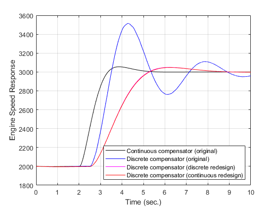
Plot the responses of the design. The redesign of the control system using both approaches yields similar controllers. This example shows the effects of the computational delay and discretization. These effects reduce the stability margins of the system, but when you properly model a control system you can achieve the desired closed-loop behavior.

plot(T1,Y1,'k',T3,Y3,'b',Td,Yd,'m',Tc,Yc,'r')
xlabel('Time (sec.)')
ylabel('Engine Speed Response')
legend('Continuous compensator (original)','Discrete compensator (original)', ...
    'Discrete compensator (discrete redesign)',...
    'Discrete compensator (continuous redesign)',...
    'Location','southeast');
grid

bdclose('scdspeed_contcomp')
bdclose('scdspeed_compdelay')