Specify Linearization for Model Components Using System Identification

Linearize Hard Drive Model

Open the Simulink® model for the hard drive.

model = 'scdpwmharddrive';
open_system(model)

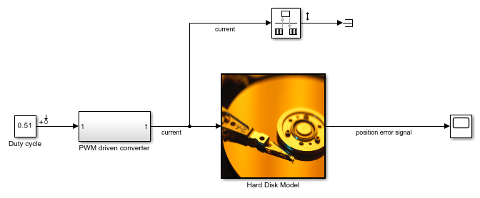
In this model, the hard drive plant is driven by a current source. The current source is implemented by a circuit that is driven by a pulse width modulation (PWM) signal so that its output can be adjusted by the duty cycle. For details of the hard drive model, see Digital Servo Control of a Hard-Disk Drive.

PWM-driven circuits usually have high frequency switching components, such as the MOSFET transistor in this model, whose average behavior is not well defined. Therefore, finding an exact linearization of this type of circuit is problematic. When you linearize the model from the duty cycle input to the position error, the result is zero.

The Simscape solver in this model is configured to run in local solver mode, which is not supported for linearization. Therefore, turn off the local solver when linearizaing the model.

SimscapeSolver = [model '/PWM driven converter/Solver Configuration'];
set_param(SimscapeSolver,'UseLocalSolver','off')

Linearize the model.

io(1) = linio('scdpwmharddrive/Duty cycle',1,'input');
io(2) = linio('scdpwmharddrive/Hard Disk Model',1,'output');
sys = linearize(model,io)

sys =
 
  D = 
                 Duty cycle
   position err           0
 
Static gain.

As expected, the PWM components cause the system to linearize to zero.

Turn the local solver back on for simulation.

set_param(SimscapeSolver,'UseLocalSolver','on')

Find Linear Model for PWM Component

You can estimate the frequency response of the PWM-driven current source and use the result to identify a linear model.

The current signal has a discrete sample time of 1e-7. Therefore, you need to use a sinestream signal with a fixed sample time as your estimation input signal. Create a signal that has frequencies between 2,000 and 200,000 rad/s.

idinput = frest.createFixedTsSinestream(Ts,{2000,200000});
idinput.Amplitude = 0.1;

Define the input and output points for the PWM-driven circuit, and run the frequency response estimation using the sinestream input signal.

pwm_io(1) = linio('scdpwmharddrive/Duty cycle',1,'input');
pwm_io(2) = linio('scdpwmharddrive/PWM driven converter',1,'openoutput');
sysfrd = frestimate(model,pwm_io,idinput);

To identify a second-order model using the frequency response data, use the System Identification Toolbox function tfest.

sysid = ss(tfest(idfrd(sysfrd),2));

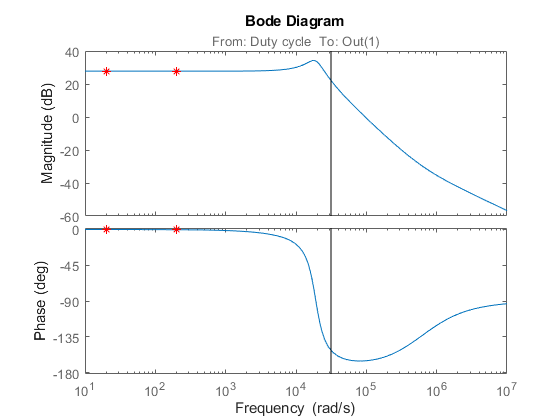
Compare the identified model to the original frequency response data.

bode(sysid,sysfrd,'r*')

To estimate the frequency response, you used frequencies between 2,000 and 200,000 rad/s. The identified model has a flat magnitude response for frequencies smaller than 2,000 rad/s. However, the previous estimation did not include those frequencies.

To verify whether the frequency response is flat for lower frequencies, estimate the response using a sinestream input signal with frequencies of 20 and 200 rad/s.

lowfreq = [20 200];
inputlow = frest.createFixedTsSinestream(Ts,lowfreq)

 
The sinestream input signal:
 
      Frequency           : [20 200] (rad/s)
      Amplitude           : 1e-05
      SamplesPerPeriod    : [3141593 314159]
      NumPeriods          : 4
      RampPeriods         : 0
      FreqUnits (rad/s,Hz): rad/s
      SettlingPeriods     : 1
      ApplyFilteringInFRESTIMATE (on/off)    : on
      SimulationOrder (Sequential/OneAtATime): Sequential
 

The combination of the fast sample time of 1e-7 seconds (10 MHz sampling frequency) and the lower frequencies creates high SamplesPerPeriod values for the input signal. In this case, considering that each frequency has four periods, frequency response estimation would log output data with around 14 million samples.

Since such a high sampling rate is not necessary for analyzing 20 and 200 rad/s frequencies, you can avoid memory issues by increasing the sample time to 1e-4.

Tslow = 1e-4;
wslow = 2*pi/Tslow;
inputlow = frest.createFixedTsSinestream(Tslow,wslow./round(wslow./lowfreq));
inputlow.Amplitude = 0.1;

To make the model compatible with the smaller sample time, resample the output data point using a rate transition block as in the modified model.

modellow = 'scdpwmharddrive_lowfreq';
open_system(modellow)

You can estimate a frequency response for the low frequencies using the following command.

sysfrdlow = frestimate(modellow,getlinio(modellow),inputlow);

The frequency response estimation can take several minutes. For this example, load the estimation results.

load scdpwmharddrive_lowfreqresults

To validate the low-frequency response of the identified model, compare the estimated result with the identified model.

bode(sysid,sysfrdlow,'r*')

Close the low-frequency model.

bdclose(modellow)

Specify Linearization for PWM Component

To specify the linearization of the PWM-driven component using the validated identified model, specify the linearization of the PWM-driven converter subsystem.

To do so, first enable block linearization specification for the converter block.

pwmblock = 'scdpwmharddrive/PWM driven converter';
set_param(pwmblock,'SCDEnableBlockLinearizationSpecification','on');

Specify sysid as the block linearization using a MATLAB® expression.

rep = struct('Specification','sysid',...
             'Type','Expression',...
             'ParameterNames','',...
             'ParameterValues','');
set_param(pwmblock,'SCDBlockLinearizationSpecification',rep);

Set the sample time of the duty cycle reference signal to that of the plant.

set_param('scdpwmharddrive/Duty cycle','SampleTime','Ts_plant');

Linearize the model. Disable the local solver during linearation.

set_param(SimscapeSolver,'UseLocalSolver','off')
sys = linearize(model,io);
set_param(SimscapeSolver,'UseLocalSolver','on')

You can validate the overall linearization result by estimating the frequency response using the following commands.

valinput = frest.Sinestream(sys);
valinput = fselect(valinput,3e3,1e5);
valinput.Amplitude = 0.1;
sysval = frestimate(model,io,valinput);

The frequency response estimation can take several minutes. For this example, load the estimation results.

load scdpwmharddrive_valfreqresults
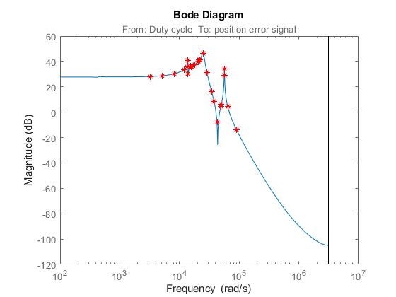
bodemag(sys,sysval,'r*')

The linearization result is accurate and all the resonances exist in the actual dynamics of the model.