Estimate Parameters from Measured Data
About This Tutorial
Objectives
This tutorial shows how to estimate parameters of a single-input single-output (SISO) Simulink® model from measured input and output (I/O) data.
Note
Simulink Design Optimization™ software estimates parameters from real, time-domain data only.
You can perform the following tasks using the Parameter Estimator:
Load a saved session containing data
Estimate model parameters using default settings
Validate the model, and refine the estimation results
Engine Throttle Model
Open the engine throttle system model.
open_system('spe_engine_throttle1.slx')About the Model
This example uses the spe_engine_throttle1
Simulink model, which represents an engine throttle system.
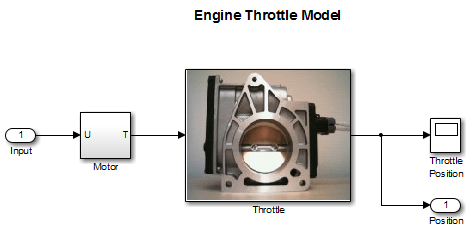
The throttle system controls the flow of air and fuel mixture to the engine cylinders. The throttle body contains a butterfly valve that opens when a driver presses the accelerator pedal. Opening this valve increases the amount of fuel mixture entering the cylinders, which increases the engine speed. A DC motor controls the opening angle of the butterfly valve in the throttle system. The models for these components are described in Motor Subsystem and Throttle Subsystem.
The input to the throttle system is the motor current (in amperes), and the output is the angular position of the butterfly valve (in degrees).
Motor Subsystem. The Motor subsystem contains the DC motor model. To
open the model, double-click the corresponding block.

Components of the Motor
subsystem | Description |
|---|---|
| Variables | U is the input current to the motor. T is the torque applied by the motor. |
| Parameters |
|
| Equation | The torque applied by the motor is described in the following equation: where t is time. |
| Input | U |
| Output | T |
Throttle Subsystem. The Throttle subsystem contains the butterfly valve
model. To open the model, right-click the corresponding block, and select View Mask > Look Under Mask.

The Hard Stops block models the valve angular position
limit of 15° to 90°.
The following table describes the variables, parameters, states, differential equations, inputs, and outputs of the throttle model.
Components of the
Throttle subsystem | Description |
|---|---|
| Variables | T is the torque applied by the DC motor. θ is the
angular position of the valve, represented by
Thardstop is the torque applied by the hard stop. |
| Parameters |
|
| States | is the angular position. is the angular velocity. |
| Equations | The mathematical system for the butterfly valve is described in the following equation: where , with initial conditions , and . The torque applied by the
where |
| Input | T |
| Output | θ |
Estimate Model Parameters Using Default Estimation Settings
Overview of the Estimation Process
Simulink Design Optimization software uses optimization techniques to estimate model parameters. In each optimization iteration, it simulates the model with the current parameter values. It computes and minimizes the error between the simulated and measured output. The estimation is complete when the optimization method finds a local minimum.
To start the estimation process, first open the Parameter Estimator app from the Simulink model.
In the Simulink Toolstrip, on the Apps tab, under Control Systems, select Parameter Estimator.
This action opens a new session with the name Parameter Estimation - spe_engine_throttle1 in the Parameter Estimator.
Note
The Simulink model must remain open to perform parameter estimation tasks.
Specify Estimation Data and Parameters
Load or import the estimation data.

If you prepared data and saved your session as described in Prepare Data for Parameter Estimation, load the preconfigured session. On the Parameter Estimation tab, click the
Open
                                        Session
drop down list.
Select the correct option to browse to the location of your saved session, for example,
Open from
                                        file
. Then select the MAT file.If you do not have a previously saved session, create a new experiment. on the Parameter Estimation tab, click New Experiment. In the Experiments list on the left pane. You can rename it by right-clicking and selecting Rename from the list. For example, call it
NewData1.To import data into the experiment, right-click and select Edit... to launch the experiment editor. Import the output data by typing in the dialog box in the Outputs panel, for example
[time1,position1]. Import the input data by typing in the dialog box in the Inputs panel, for example[time1,input1].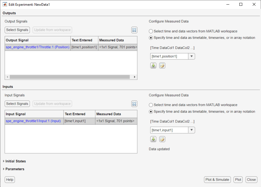
You can also specify the relative importance of each data point in an output data signal with respect to other data points in the same output data signal. To do this, click the output signal for which you want to specify weights. In the Signal Weights menu, you can either choose a variable defined in the base workspace as the signal weights or manually enter the weights as scalars or vectors.
For more information, see Edit Experiment Data.
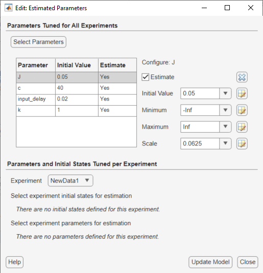
Specify parameters for estimation. On the Parameter Estimation tab, click the Select Parameters button to open the Edit: Estimated Parameters dialog box. In the Parameters Tuned for all Experiments panel, click the Select parameters button to launch the Select Model Variables dialog box.
Select the parameters
J,c,input_delay, andk, and click OK.Note
In your application, if the model parameters you want to estimate are not listed in the Select Model Variables dialog box, first specify these parameters as variables. See, Add Model Parameters as Variables for Estimation.

The Edit: Estimated Parameters window now looks as follows.

The app selects the parameters you add for estimation by default. When estimating a large number of parameters, you can first select a subset of parameters to estimate.
You can also first use sensitivity analysis to identify the parameters that most influence the estimation, and then specify these parameters for estimation. To open the Sensitivity Analyzer, in the Parameter Estimation tab, click
 Sensitivity
Analysis. In the Sensitivity Analyzer, you can
identify the model parameters that most influence the estimation problem
and compute initial values for the estimation parameters.
Sensitivity
Analysis. In the Sensitivity Analyzer, you can
identify the model parameters that most influence the estimation problem
and compute initial values for the estimation parameters.Specify an experiment for estimation. On the Parameter Estimation tab, click Select Experiments, and select the box under the Estimation column. Click OK.
To add progress plots, click Add Plot on the Parameter Estimation tab. Here you can choose the Parameter Trajectory and Estimation Cost iteration plots. You can also choose an experiment plot of measured and simulated data for
NewData1.Estimate the parameters using the default settings. On the Parameter Estimation tab, click Estimate to open the Parameter Trajectory plot and Estimation Progress Report window and estimate the parameters. The Parameter Trajectory plot shows the change in the parameter values at each iteration.

The Estimation Progress Report shows the iteration number, number of times the objective function is evaluated, and the value of the cost function at the end of each iteration. After the estimation converges, the Estimation Progress Report looks like this figure.

The estimated parameters are saved in the Parameter Estimator, in the Results section of the Data Browser pane, as
EstimatedParams. Right-clickEstimatedParams, and select Open... to view the results.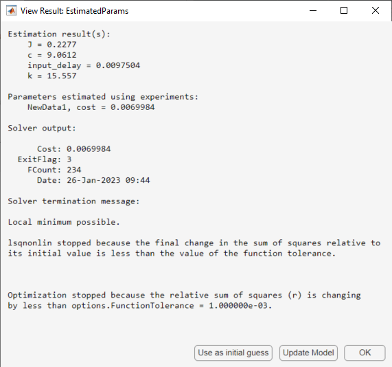
Examine the estimated cost function graph. Cost function is the error between the simulated and measured output. During estimation, the default optimization method
Nonlinear least squares,lsqnonlin, minimizes the cost function by changing the parameter values. The following figure displays the change in the expected cost during iterations.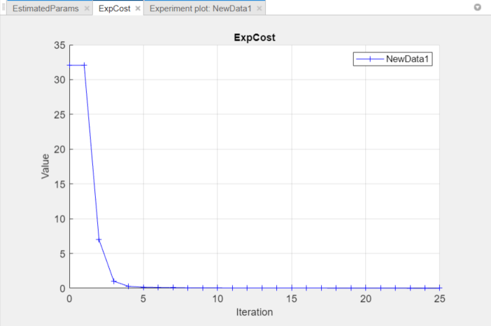
Examine the simulated response plot to see how well the simulated output matches the measured output. The experiment plot shows that the output simulated using the estimated parameters is close to the measured outputs.

Improve Estimation Results Using Parameter Bounds
You can improve the accuracy of estimation by specifying bounds on parameter values. This technique restricts the region in which the optimization method searches for a local minima.
The engine throttle system has these characteristics:
All parameter values are positive.
Maximum time delay of the system, represented by
input_delay, is 0.1 s.
Therefore, specify 0 as the minimum value for all parameters, and 0.1
as the maximum value of input_delay. In the Parameter
Estimator, click the Select Parameters button to
specify bounds on the parameter values. For each parameter, click the right
parameter to display the minimum, maximum, and scale fields. Specify the minimum
value for each parameter by replacing -Inf with
0 in the Minimum field. Specify the
maximum value for input_delay by replacing
+Inf with 0.1 in the corresponding
Maximum field.

After estimating the parameters, analyze the results using the experiment plot and the plot for expected cost.

The data simulated using the estimated parameter values agree better with the measured data than when the parameter limits were not specified.

Validate Estimated Model Parameters
After estimating model parameters, validate the model using another data set (validation data). A good match between the simulated response and the validation data indicates that you have not overfitted the model.
To validate the estimated parameters using a validation data set:
Create a new experiment to use for validation. Name it
ValidationData. Import the validation I/O data,input2andposition2, and the time vector,time2in theValidationDataexperiment. To do this, in the Parameter Estimator, in the Experiments pane, right-clickValidationDataand select Edit... to open the experiment editor. Then, type[time2,position2]in the output dialog box and[time2,input2]in the input dialog box. For more information, see Import Data for Parameter Estimation.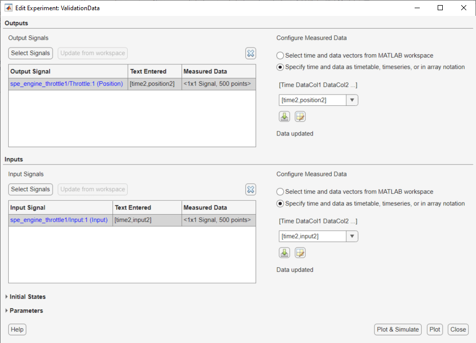
Select the experiment for validation. On the Parameter Estimation tab, click Select Experiments. By default, the
ValidationDataexperiment is selected for estimation. Deselect the check box that corresponds toValidationDatafor estimation and select the check box for validation.
Select results to use. On the Validation tab, click Select Results to Validate.

Deselect
Use current parameter valuesand selectEstimatedParams, and click OK.Select the plots for measured and simulated data, and residuals on the Validation tab. You can assess how much the data simulated using the estimated parameters agrees with the measured data using these plots.

On the Validation tab, click Validate to start validation.
Examine the plots.
Examine the experiment plot to see how well the simulated output matches the output data.

The simulated response as shown in light brown on the top experiment plot is overlaid on the measured out put data, and closely matches the measured validation data.
Examine the residuals plot to compare the difference between the simulated response and measured data.

The difference between the simulated and measured data varies between 2 and -2.5. The residuals lie within 6% of the maximum output variation and do not display any systematic patterns. This indicates a good fit between the simulated output and measured data.
Save the session. On the Parameter Estimation tab, click Save Session.
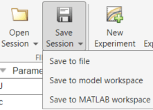
From the drop-down list select where to save the session. Specify the file name, and click Save or OK to save your parameter estimation session as a MAT file.