Prepare Data for Parameter Estimation
About This Tutorial
Objectives
This tutorial explains how to import, analyze, and prepare measured input and output (I/O) data for estimating parameters of a Simulink® model.
Note
Simulink Design Optimization™ software estimates parameters from real, time-domain data only.
Perform the following tasks using the Parameter Estimator:
Import data from the MATLAB® workspace.
Analyze data quality using a time plot.
Select a subset of data for estimation.
Replace outliers.
Filter high-frequency noise.
About the Sample Data
Load spe_engine_throttle1.mat, which contains I/O data
measured from an engine throttle system. The MAT file includes the following
variables:
input1— Input data samplesposition1— Output data samplestime1— Time vector
Note
The number of input and output data samples must be equal to the length of the corresponding time vector.
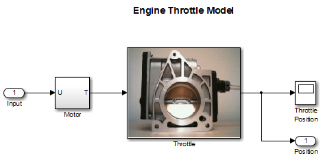
The engine throttle system controls the flow of air and fuel mixture to the engine cylinders. The throttle body contains a butterfly valve which opens when a driver presses the accelerator pedal. Opening this valve increases the amount of fuel mixture entering the cylinders, which increases the engine speed. A DC motor controls the opening angle of the butterfly valve in the throttle system. The input to the throttle system is the motor current (in amperes), and the output is the angular position of the butterfly valve (in degrees).
spe_engine_throttle1 contains the Simulink model of the engine throttle system.
Engine Throttle Model
Open the engine throttle system model.
open_system('spe_engine_throttle1.slx')Start a Parameter Estimator Session
To perform parameter estimation, you must first start a Parameter Estimator session.
When you open the Simulink model, the model loads the data into the MATLAB workspace.

In the Simulink model window, on the Apps tab, under Control Systems, select Parameter Estimator.
This action opens a new session, Parameter Estimation - spe_engine_throttle1, in the Parameter Estimator.

Note
The Simulink model must remain open to perform parameter estimation tasks.
Create an Experiment for Parameter Estimation
In the Parameter Estimator on the Parameter
Estimation tab, click the New Experiment
button. This will create an experiment with the name Exp in the
Experiments list on the left pane. To rename it,
right-click it and select Rename from the list. For example,
call it NewData1.
Import Data
This portion of the tutorial explains how to import measured I/O data into the experiment in the Parameter Estimator. Importing data assigns the data to the corresponding model input and output signals.
The model input and output signals are designated with the Inport
Input and Outport Position blocks,
respectively. To learn more about the blocks, see the Inport and Outport block reference pages in
the Simulink documentation.
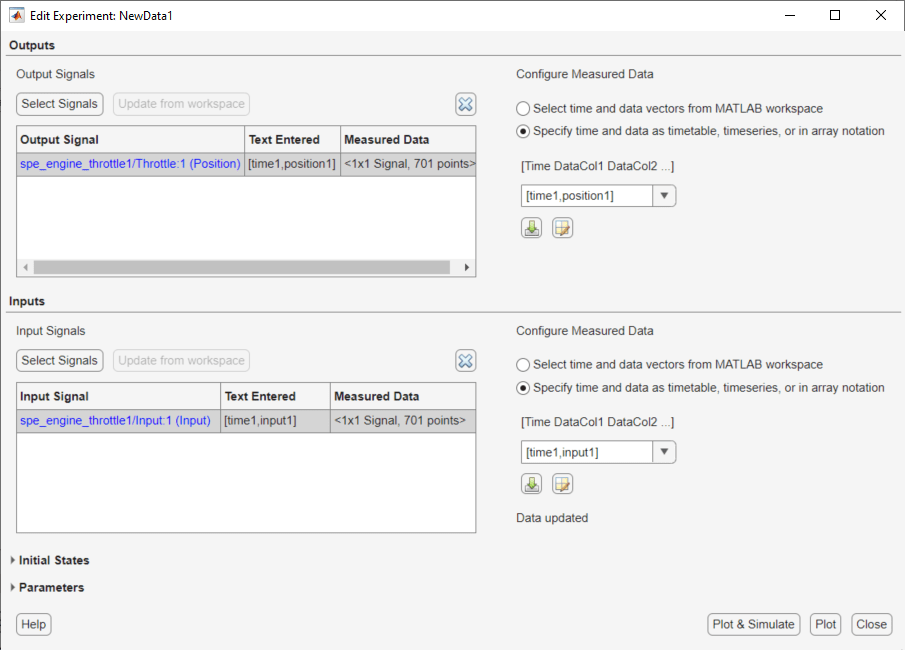
To import data into the experiment, right-click and select
Edit... to launch the experiment editor. Import the
output data by typing [time1,position1] in the dialog box in the
Outputs panel. Import the input data by typing
[time1,input1] in the dialog box in the
Inputs panel.

Analyze Data
This portion of the tutorial explains how to analyze the output data quality by viewing the data characteristics on a time plot. Based on the analysis, you can decide whether to preprocess the data before estimating parameters. For example, if the data contains noise, you might want to filter the noise from the system dynamics before estimating parameters.
To create an experiment plot, click Add Plot on the
Parameter Estimation tab and select the experiment name,
for example, NewData1 under Experiment Plots.

The time plot shows the output data in response to a step input, as described in About the Sample Data. The plot shows a rapid decrease in the response after t = 0.5 s because the system is shut down. To focus parameter estimation on the time period when the system is active, select the data samples between t = 0 s and t = 0.5 s, as in Extract Data for Estimation.
The spikes in the data indicate outliers, defined as data values that deviate from the mean by more than three standard deviations. They might be caused by measurement errors or sensor problems. The response also contains noise. Before estimating model parameters from this data, remove the outliers and filter the noise, as described in Replacing Outliers and Filtering Data.
You can also plot the experiment data by right-clicking the experiment, for
example NewData1, and selecting Plot measured
experiment data from the list.
Extract Data for Estimation
This portion of the tutorial explains how to select a subset of I/O data for estimation. As described in Analyze Data, the system is shut down at t = 0.5 s. To focus the estimation on the time period before t = 0.5 s, exclude the data samples beyond t = 0.5 s. This operation selects the data between t = 0 s and t = 0.5 s for estimation.
First, import the data into the experiment, as described in Import Data.
To select the portion of data between t = 0 s and t = 0.5 s:
Plot the measured data as described in Analyze Data, to have access to the Experiment Plot tab.
On the Experiment Plot tab, click Extract Data to launch the Extract Data tab.
Enter 0 in the Start Time: field and 0.5 in the End Time: field.
Click Save As to save data in a new experiment, for example,
NewData1_1.
The Parameter Estimator extracts the corresponding input data. To plot
the new data, click on Add Plot on the Parameter
Estimation tab. Select the experiment name, for example,
NewData1_1 in the Experiment Plots list
to display the experiment plot of the data from t = 0 s to t = 0.5 s.

Replacing Outliers
Why Replace Outliers
Outliers are data values that deviate from the mean by more than three standard deviations. When estimating parameters from data containing outliers, the results might not be accurate. Hence, you might choose to replace the outliers in the data before you estimate the parameters.
How to Replace Outliers
In the experiment plot of the data extracted as in Extract Data for Estimation, you can visually detect the data points that seem to be outliers. To replace these points:
In the Experiment Plot tab, click Replace data to launch the Replace data tab. The experiment plot shows the preview data. On the preview, select the data point that you want to replace.
On the Replace Data tab, click Replace data and select the constant value. For example, replace the output signal data that correspond to time points 0.00899 and 0.0189 with 15, that corresponds to the time point 0.149 with 86, and the rest of the outlier data points with 90.
Click the arrow in the Apply section and select Save As: Create a new experiment from the modified data. Parameter Estimator saves the modified data in the new experiment, for example,
NewData1_1_1.Click Add Plot on the Parameter Estimation tab and select the new experiment, for example,
NewData1_1_1. This creates an experiment plot of the modified data. The spikes, that indicated outliers, no longer appear on the time plot.
Filtering Data
This portion of the tutorial explains how to filter the noise and remove any periodic trends from the output data. First remove the outliers from the output data, as described in Replacing Outliers.
Click the experiment plot for the new experiment, for example,
NewData1_1_1. On the Experiment Plot
tab, click Low-Pass Filter.
On the Low-Pass Filter tab select Filter all signals.
Enter 0.4 in the Normalized cutoff frequency field.
Click Options. Enter 1 in the Filter order field.

Click the arrow in the Apply section and select Save As: Create a new experiment from the modified data. Parameter Estimator saves the modified data in the new experiment, for example,
NewData1_1_1_1.Click Add Plot on the Parameter Estimation tab and select the new experiment,
NewData1_1_1_1. This creates an experiment plot of the modified data. The noise is filtered and the output data appears smooth.
Saving the Session
After you prepare the data, delete the data in the older experiments, for example,
New Data1, New Data1_1, New
Data1_1_1. You can rename the last experiment, for example,
NewData1_1_1_1 as NewData1, and save the
session.
To delete the experiments, right-click the experiment name in the Experiments pane, and select Delete from the list.
To save the session, click Save Session on the
Parameter Estimation tab to select where to save the
session. Specify a name for the session, for example,
spe_engine_throttle1_sdosession.mat in the File
name or Session field, and then click
Save or OK. This saves your
parameter estimation session as a MAT file.
To learn how to estimate parameters from this data, see Estimate Parameters from Measured Data.