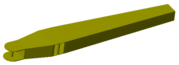
Model an Excavator Dipper Arm as a Flexible Body

Step 1: Define the Geometry and Material Properties of the Dipper Arm

The file Dipper.STL contains a triangulation that defines the CAD geometry of the dipper arm. To view the geometry stored in this file, use the MATLAB® functions stlread and trisurf:

stlFile = 'Dipper.STL';
figure
trisurf(stlread(stlFile))
axis equal

The dipper arm is constructed from steel. To represent its material properties, set these values for Young's modulus, Poisson's ratio, and mass density:

E = 200e9;     % Young's modulus in Pa
nu = 0.26;     % Poisson's ratio (nondimensional)
rho = 7800;    % Mass density in kg/m^3

Step 2: Specify the Locations of Interface Frames

The dipper arm has three interface frames where you can connect other Simscape™ Multibody™ elements, such as joints, constraints, forces, and sensors:

The positions of all interface frame origins are specified in meters relative to same common reference frame used by the CAD geometry.

origins = [-0.500  0      0      % Frame 1: Cylinder connection point
            1.500  0      0      % Frame 2: Bucket connection point
            0     -0.130  0];    % Frame 3: Fulcrum point
numFrames = size(origins,1);

Step 3: Create the Finite-Element Mesh

To generate the mesh for the dipper arm, first call the createpde (Partial Differential Equation Toolbox) function, which creates a structural model for modal analysis of a solid (3-D) problem. After importing the geometry and material properties of the arm, the generateMesh (Partial Differential Equation Toolbox) function creates the mesh.

feModel = createpde('structural','modal-solid');
importGeometry(feModel,stlFile);
structuralProperties(feModel, ...
    'YoungsModulus',E, ...
    'PoissonsRatio',nu, ...
    'MassDensity',rho);
generateMesh(feModel, ...
    'GeometricOrder','quadratic', ...
    'Hmax',0.2, ...
    'Hmin',0.02);

Step 4: Set up the Multipoint Constraints for the Interface Frames

Each interface frame on the block corresponds to a boundary node that contributes six degrees of freedom to the reduced-order model. There are several ways to ensure that the FEA substructuring method preserves the required degrees of freedom. For example, you can create a rigid constraint to connect the boundary node to a subset of finite-element nodes on the body. You can also use structural elements, such as beam or shell elements, to introduce nodes with six degrees of freedom.

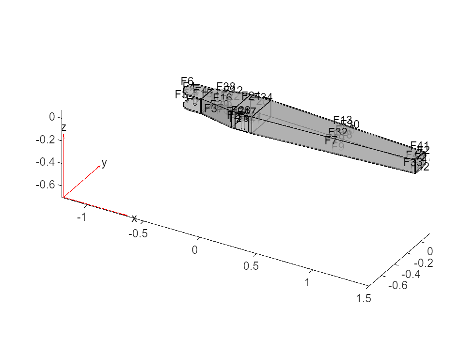
This example uses a multipoint constraint (MPC) to preserve the six degrees of freedom at each boundary node. To identify the geometric regions (such as faces, edges, or vertices) to associate with each MPC, first plot the arm geometry by using the function pdegplot (Partial Differential Equation Toolbox):

figure
pdegplot(feModel,'FaceLabels','on','FaceAlpha',0.5)

You can zoom, rotate, and pan this image to determine the labels for the faces corresponding to the boundary nodes. These faces define the MPCs associated with the boundary nodes in the dipper arm:

faceIDs = [1,27,23];    % List in the same order as the interface frame origins

To verify these values, plot the mesh and highlight the selected faces:

figure
pdemesh(feModel,'FaceAlpha',0.5)
hold on
colors = ['rgb' repmat('k',1,numFrames-3)];
assert(numel(faceIDs) == numFrames);
for k = 1:numFrames
    nodeIdxs = findNodes(feModel.Mesh,'region','Face',faceIDs(k));
    scatter3( ...
        feModel.Mesh.Nodes(1,nodeIdxs), ...
        feModel.Mesh.Nodes(2,nodeIdxs), ...
        feModel.Mesh.Nodes(3,nodeIdxs), ...
        'ok','MarkerFaceColor',colors(k))
    scatter3( ...
        origins(k,1), ...
        origins(k,2), ...
        origins(k,3), ...
        80,colors(k),'filled','s')
end
hold off

Call the function structuralBC (Partial Differential Equation Toolbox) to define the MPCs for the boundary nodes in these faces:

for k = 1:numFrames
    structuralBC(feModel, ...
        'Face',faceIDs(k), ...
        'Constraint','multipoint', ...
        'Reference',origins(k,:));
end

Step 5: Generate the Reduced-Order Model

The function reduce (Partial Differential Equation Toolbox) applies the Craig-Bampton order reduction method and retains all fixed-interface modes up to a frequency of $$10^4$$ radians per second.

rom = reduce(feModel,'FrequencyRange',[0 1e4]);

Store the results of the reduction in a data structure arm. Transpose the ReferenceLocations matrix to account for the different layout conventions used by Partial Differential Equation Toolbox and Simscape Multibody.

arm.P = rom.ReferenceLocations';  % Interface frame locations (n x 3 matrix)
arm.K = rom.K;                    % Reduced stiffness matrix
arm.M = rom.M;                    % Reduced mass matrix

The function computeModalDampingMatrix, which is defined at the bottom of this page, computes a reduced modal damping matrix with a damping ratio of 0.05:

dampingRatio = 0.05;
arm.C = computeModalDampingMatrix(dampingRatio,rom.K,rom.M);

The boundary nodes in the reduced-order model must be specified in the same order as the corresponding interface frames on the block. This order is given by the rows of the array origins. If the order of the MPCs is different than the order specified by origins, permute the rows and columns of the various matrices so that they match the original order.

frmPerm = zeros(numFrames,1);    % Frame permutation vector
dofPerm = 1:size(arm.K,1);       % DOF permutation vector

assert(size(arm.P,1) == numFrames);
for i = 1:numFrames
    for j = 1:numFrames
        if isequal(arm.P(j,:),origins(i,:))
            frmPerm(i) = j;
            dofPerm(6*(i-1)+(1:6)) = 6*(j-1)+(1:6);
            continue;
        end
    end
end
assert(numel(frmPerm) == numFrames);
assert(numel(dofPerm) == size(arm.K,1));

arm.P = arm.P(frmPerm,:);
arm.K = arm.K(dofPerm,:);
arm.K = arm.K(:,dofPerm);
arm.M = arm.M(dofPerm,:);
arm.M = arm.M(:,dofPerm);
arm.C = arm.C(dofPerm,:);
arm.C = arm.C(:,dofPerm);

Step 6: Import Reduced-Order Data

The model ReducedOrderFlexibleSolid uses the data structure arm to set up the parameters of the Reduced Order Flexible Solid block. In the block, these parameters import the reduced-order data:

For more information, see Using the Reduced Order Flexible Solid Block - Flexible Dipper Arm.

Compute the Modal Damping Matrix

This function computes a modal damping matrix associated with the stiffness matrix K and mass matrix M. This function applies a single scalar damping ratio to all of the flexible (non-rigid-body) normal modes associated with K and M.

function C = computeModalDampingMatrix(dampingRatio,K,M)

% To avoid numerical issues (such as complex eigenvalues with very small
% imaginary parts), make the matrices exactly symmetric.

    K = (K+K')/2;    % Stiffness matrix
    M = (M+M')/2;    % Mass matrix

% Compute the eigen-decomposition associated with the mass and stiffness
% matrices, sorting the eigenvalues in ascending order and permuting
% the corresponding eigenvectors.

    [V,D] = eig(K,M);
    [d,sortIdxs] = sort(diag(D));
    V = V(:,sortIdxs);

% Due to small numerical errors, the six eigenvalues associated with the
% rigid-body modes may not be exactly zero. To avoid numerical issues,
% check that the first six eigenvalues are close enough to zero. Then
% replace them with exact 0 values.

    assert(all(abs(d(1:6))/abs(d(7)) < 1e-9),'Error due to "zero" eigenvalues.');
    d(1:6) = 0;

% Vectors of generalized masses and natural frequencies

    MV = M*V;
    generalizedMasses = diag(V'*MV);
    naturalFrequencies = sqrt(d);

% Compute the modal damping matrix associated with K and M

    C = MV * diag(2*dampingRatio*naturalFrequencies./generalizedMasses) * MV';

end