Analyze a Simple Circuit

Introduction

In this section, you

Obtain the state-space representation of your model with the power_analyze command
Compute the steady-state voltages and currents using the graphical user interface of the Powergui block
Analyze an electrical circuit in the frequency domain

Electrical State Variables

The electrical state variables are the Simulink^® states of your diagram associated to the capacitor and inductor devices of the Simscape™ Electrical™ Specialized Power Systems blocks. Inductors and capacitors elements are found in the RLC-branch type blocks such as the Series RLC Branch block, Three-Phase Parallel RLC Load block, in the transformer models, in the PI Section Line block, in the snubber devices of the power electronic devices, etc.

The electrical state variables consist of the inductor currents and the capacitor voltages. Variable names for Simscape Electrical Specialized Power Systems electrical states contain the name of the block where the inductor or capacitor is found, preceded by the Il_ prefix for inductor currents or the Uc_ prefix for capacitor voltages.

State-Space Representation Using power_analyze

You compute the state-space representation of a model with the power_analyze command. Enter the following command at the MATLAB^® prompt.

[A,B,C,D,x0,electrical_states,inputs,outputs]=power_analyze('power_gui')

The power_analyze command returns the state-space model of power_gui example model in the four matrices A, B, C, and D. x0 is the vector of initial conditions of the electrical states of your circuit. The names of the electrical state variables, inputs, and outputs are returned in three matrices.

See the power_analyze reference page for more details on how to use this function.

Steady-State Analysis

Open the power_gui example model by typing power_gui at the command line. Then open the Powergui block and, in the Apps tab, select Measurement and States Analyzer to display the steady-state phasor voltages measured by the voltage measurement and current measurement blocks of the model.

Each measurement output is identified by a character vector corresponding to the measurement block name. The magnitudes of the phasors correspond to the peak value of the sinusoidal voltages.

You can also display the steady-state values of the source voltage or the steady-state values of the inductor currents and capacitor voltages by selecting either the Sources or the States check box.

Refer to the section Measuring Voltages and Currents for more details on the sign conventions used for the voltages and currents of sources and electrical state variables listed in the Measurement and States Analyzer app window.

Frequency Analysis

The Simscape > Electrical > Specialized Power Systems > Sensors and Measurements library contains an Impedance Measurement block that measures the impedance between any two nodes of a circuit. In the following two sections, you measure the impedance in the power_gui model by using two methods:

Automatic measurement using the Impedance Measurement block and the Powergui block
Calculation from the state-space model

Obtaining the Impedance vs. Frequency Relation from the Impedance Measurement and Powergui Blocks

The process to measure a circuit impedance from the state-space model (which is described in detail in the next section, Obtaining the Impedance vs. Frequency Relation from the State-Space Model) has been automated in a Simscape Electrical Specialized Power Systems block. In the power_gui example model, two Impedance Measurement blocks of powerlib measure impedance at two points in the model. Delete the Impedance B3 block and reconnect the Impedance B1 as shown.

Measuring Impedance vs. Frequency with the Impedance Measurement Block

In the 150 km Line block, set Number of pi sections to 1, and click OK. Open the Powergui dialog. In the Apps tab, select Impedance Calculator. A new window opens, showing the list of Impedance Measurement blocks available in the circuit.

Fill in the frequency range by entering 0:2:5000 (zero to 5000 Hz by steps of 2 Hz). Select the logarithmic scale to display Z magnitude.

When the calculation is finished, the window displays the magnitude and phase as functions of frequency. In the 150 km Line block dialog box, set the Number of pi sections to 10. In the Powergui Impedance Calculator tool, click the Update button. The block dialog box displays the frequency response for the new circuit.

Obtaining the Impedance vs. Frequency Relation from the State-Space Model

Note

The following section assumes that you have Control System Toolbox™ software installed.

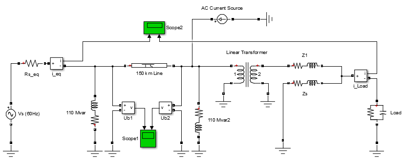
To measure the impedance versus frequency at the same node where the impedance measurement block is connected, you need a current source providing a second input to the state-space model. Add the AC Current Source block from the Simscape > Electrical > Specialized Power Systems > Sources library to your model. Connect this source, as shown below. Set the current source magnitude to zero and keep its frequency at 60 Hz.

AC Current Source at the B2 Node

Now compute the state-space representation of the model with the power_analyze command. Enter the following command at the MATLAB prompt.

sys1 = power_analyze('power_gui','ss')

This command returns a state-space model representing the continuous-time state-space model of your electrical circuit.

In the Laplace domain, the impedance is defined as the transfer function between the current injected by the AC current Source block and the voltage measured by the U2 Voltage Measurement block.

$Z 2 (s) = \frac{U 2 (s)}{I 2 (s)}$

You obtain the names of the inputs and outputs of this state-space model as follows.

sys1.InputName
ans = 
    'U_Vs (60Hz)'
    'I_AC Current Source'
sys1.OutputName
ans = 
    'U_Ub2'
    'U_Ub1'

The impedance at the measured node then corresponds to the transfer function between output 1 and input 2 of this state-space model. For the 0–5000 Hz range, it can be calculated and displayed as follows.

freq=0:5000;
w=2*pi*freq;
bode(sys1(1,2),w);

Repeat the same process to get the frequency response with a 10 section line model. Open the PI Section Line dialog box and change the number of sections from 1 to 10. To calculate the new frequency response and superimpose it upon the one obtained with a single line section, enter the following commands.

sys10 = power_analyze('power_gui','ss');
bode(sys1(1,2),sys10(1,2),w);

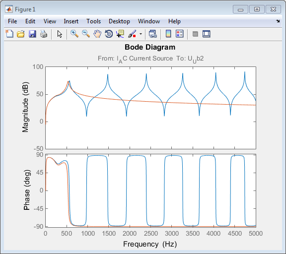
Open the property editor of the Bode plot and select units for Frequency in Hz using linear scale and Magnitude in absolute using log scale. The resulting plot is shown below.

Impedance at the Measured Node as Function of Frequency

This graph indicates that the frequency range represented by the single line section model is limited and the 10 line section model gives a better approximation for higher frequencies.