RST Controller

Predictive control using a polynomial representation

Libraries:
Simscape / Electrical / Control / General Control

Description

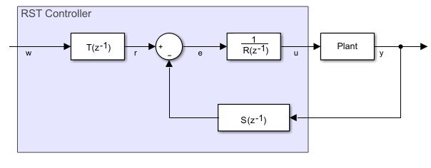
The RST Controller block implements a generalized predictive controller using a reference signal tracking polynomial representation. The diagram shows the equivalent circuit for the control algorithm.

Equations

A controlled auto-regressive integrated moving average (CARIMA) model describes the plant:

$A (z^{- 1}) y (k) = z^{- d} B (z^{- 1}) u (k - 1) + \frac{e (k) C (z^{- 1})}{D (z^{- 1})}$

$A (z^{- 1}) = 1 + a_{1} z^{- 1} + \dots + a_{n_{A}} z^{- n_{A}}$

$B (z^{- 1}) = b_{0} + b_{1} z^{- 1} + \dots + b_{n_{B}} z^{- n_{B}}$

$C (z^{- 1}) = 1$

$D (z^{- 1}) = 1 - z^{- 1},$

where:

d is the system dead-time.
y(k) is the plant output.
u(k) is the controller output.
e(k) is white noise with a zero-mean value.
A(z^-1) and B(z^-1) are the system polynomials.
n_A and n_B are the polynomials degrees.
C(z^-1) and D(z^-1) are the disturbance polynomials for obtaining the steady-state error.

The prediction model is given as

$\hat{y} (k + j | k) = G_{j - d} (z^{- 1}) D (z^{- 1}) z^{- d - 1} u (k + j) + \frac{H_{j - d} (z^{- 1}) D (z^{- 1})}{C (z^{- 1})} u (k - 1) + \frac{F_{j - d} (z^{- 1})}{C (z^{- 1})} y (k)$

and

$j = \bar{h i, h p}$

where:

hi is the minimum prediction.
hp is the prediction horizon.

The future control sequence, computed at time k, is

$u (k + j - 1 | k),$

where

$j = \bar{1, h c}$

and hc is the control horizon.

The predicted values of the output is

$\hat{y} (k + j | k) .$

To determine the system polynomials, $F_{j - d} (z^{- 1})$ , $G_{j - d} (z^{- 1})$ , and $H_{j - d} (z^{- 1})$ , the block uses two Diophantine equations. The first Diophantine equation is

$\frac{C (z^{- 1})}{A (z^{- 1}) D (z^{- 1})} = E_{j - d} (z^{- 1}) + z^{- j + d} \frac{F_{j - d} (z^{- 1})}{A (z^{- 1}) D (z^{- 1})},$

where:

$E_{j - d} (z^{- 1}) = 1 + 1 + e_{1} z^{- 1} + \dots + e_{n_{E}} z^{- n_{E}}$

$F_{j - d} (z^{- 1}) = f_{0} + f_{1} z^{- 1} + \dots + f_{n_{F}} z^{- n_{F}}$

$n_{E} = j - d - 1$

$n_{F} = max (n_{A} + n_{D} - 1, n_{C} - j + d)$

The second Diophantine equation is

$E_{j - d} (z^{- 1}) B (z^{- 1}) = C (z^{- 1}) G_{j - d} (z^{- 1}) + z^{- j + d} H_{j - d} (z^{- 1}),$

where:

$G_{j - d} (z^{- 1}) = g_{0} + g_{1} z^{- 1} + \dots + g_{n_{G}} z^{- n_{G}}$

$H_{j - d} (z^{- 1}) = h_{0} + h_{1} z^{- 1} + \dots + h_{n_{H}} z^{- n_{H}}$

$n_{G} = j - d - 1$

$n_{H} = max (n_{C}, n_{B} + d) - 1$

The resulting prediction model is

$\hat{y} (k + j | k) = G_{j - d} (z^{- 1}) D (z^{- 1}) z^{- d - 1} u (k + j) + {\hat{y}}_{0} (k + j | k),$

where

${\hat{y}}_{0} (k + j | k) = \frac{H_{j - d} (z^{- 1}) D (z^{- 1})}{C (z^{- 1})} u (k - 1) + \frac{F_{j - d} (z^{- 1})}{C (z^{- 1})} y (k)$

represents the free response of the system.

Using the matrix notation, the prediction model can be written as

$\hat{y} = {Gu}_{d} + {\hat{y}}_{0},$

where:

$\hat{y} = {[\hat{y} (k + h i | k), \hat{y} (k + h i + 1 | k), \dots, \hat{y} (k + h p | k)]}^{T}$

$G = [\begin{matrix} g_{h i - d - 1} & \dots & g_{0} & 0 & \dots & 0 \\ g_{h i - d} & \dots & g_{1} & g_{0} & \dots & 0 \\ \dots & \dots & \dots & \dots & \dots & \dots \\ g_{h c - 1} & \dots & \dots & \dots & \dots & g_{0} \\ g_{h p - d - 1} & \dots & \dots & \dots & \dots & g_{h p - h c - 1} \end{matrix}]$

$u_{d} = {[D (z^{- 1}) u (k), \dots, D (z^{- 1}) u (k + h c - 1)]}^{T}$

${\hat{y}}_{0} = {[{\hat{y}}_{0} (k + h i | k), {\hat{y}}_{0} (k + h i + 1 | k), \dots, {\hat{y}}_{0} (k + h p | k)]}^{T}$

To minimize tracking error and controller output, the block uses a cost function. To trade off between the minimization of the tracking error and the minimization of the controller output, the block uses a weighting factor, λ, such that

$J = {({Gu}_{d} + {\hat{y}}_{0} - w)}^{T} ({Gu}_{d} + {\hat{y}}_{0} - w) + λ u_{d}^{T} u_{d}$

for

$D (z^{- 1}) u (k + i) = 0$

and

$i \in [h c, h p - d - 1],$

where w is the reference trajectory vector. Minimizing the cost function, yields the equation for the optimal control sequence:

$u_{d}^{*} = (G^{T} G + λ I_{h c}) G^{T} [w - {\hat{y}}_{0}] .$

As γ_j and $j = \bar{h i, h p}$ are elements in the first row of the matrix ${(G^{T} G + λ I_{h c})}^{- 1} G^{T}$ , applying the receding horizon principle yields the control algorithm equation as

$D (z^{- 1}) u (k) = \sum_{j = h i}^{h p} γ_{j} [w (k + j | k) - {\hat{y}}_{0} (k + j | k)] .$

Substitution using ${\hat{y}}_{0} (k + j | k) = \frac{H_{j - d} (z^{- 1}) D (z^{- 1})}{C (z^{- 1})} u (k - 1) + \frac{F_{j - d} (z^{- 1})}{C (z^{- 1})} y (k)$ yields this form of the control algorithm equation:

$C (z^{- 1}) D (z^{- 1}) u (k) = - \sum_{j = h i}^{h p} γ_{j} H_{j - d} (z^{- 1}) D (z^{- 1}) u (k - 1) - \sum_{j = h i}^{h p} γ_{j} F_{j - d} (z^{- 1}) y (k) + \sum_{j = h i}^{h p} γ_{j} C (z^{- 1}) w (k + j) .$

The polynomial form of the control algorithm follows as

$R (z^{- 1}) u (k) + S (z^{- 1}) y (k) = T (z^{- 1}) w (k + h p),$

where:

$R (z^{- 1}) = (C (z^{- 1}) + \sum_{j = h i}^{h p} γ_{j} z^{- 1} H_{j - d} (z^{- 1})) D (z^{- 1}),$

$S (z^{- 1}) = \sum_{j = h i}^{h p} γ_{j} F_{j - d} (z^{- 1}),$

and

$T (z^{- 1}) = C (z^{- 1}) \sum_{j = h i}^{h p} γ_{j} z^{- h p + j} .$

Limitations

To obtain the R, S, and T polynomials, use the discrete-time instead of the continuous-time transfer function.

Examples

Buck Converter Polynomial Voltage Control

Control the output voltage of a buck converter using a polynomial RST controller. The RST controller adjusts the duty cycle. The input voltage is considered constant throughout the simulation. A variable resistor provides the load for the system. The total simulation time (t) is 0.25 seconds. At t = 0.15 seconds, the load is changed. At t = 0.2 seconds, the voltage reference is changed from 6V to 4V.

Open Model

DC Motor Control (RST)

An RST speed-control structure for a DC motor. A PWM controlled four-quadrant Chopper is used to feed the DC motor. The Control subsystem includes the RST controller with control horizon of 30, and the PWM generation. A sensor measures the rotor speed with a delay of 5ms. The total simulation time (t) is 4 seconds. At t = 1.5 seconds, the load torque increases. At t = 2.5 seconds, the reference speed is changed from 1000 rpm to 2000 rpm.

Open Model

Ports

Input

expand all

r — Plant reference
scalar

Plant system reference signal.

Data Types: single | double

y — Plant output
scalar

Plant system output signal.

Data Types: single | double

Output

expand all

u — Controller output
scalar

Control system output signal.

Data Types: single | double

Parameters

expand all

Controller parameterization — Parameterization method
`Controller polynomials` (default) | `Generate polynomials`

Method for parameterizing the controller. If you know the discrete-time R, S, and T polynomial values, select Controller polynomials. Otherwise, select Generate polynomials.

Dependencies

Selecting a parameterization method enables other parameters.

R polynomial — R polynomial values
`1` (default) | positive, scalar or vector

Vector of the R polynomials for the RST control.

Dependencies

Selecting Controller polynomials for the Controller parameterization parameter enables this parameter.

S polynomial — S polynomial values
`1` (default) | positive, scalar or vector

Vector of the S polynomials for the RST control.

Dependencies

Selecting Controller polynomials for the Controller parameterization parameter enables this parameter.

T polynomial — T polynomial values
`1` (default) | positive, scalar or vector

Vector of the T polynomials for the RST control.

Dependencies

Selecting Controller polynomials for the Controller parameterization parameter enables this parameter.

Model discrete transfer function numerator — Transfer function numerator
`1` (default) | scalar or vector

Numerator of the system discretized transfer function. To determine the discrete transfer function, if you have a license for Control System Toolbox™, use the c2d function.