Optimize Block Settings for Simulating with the Partitioning Solver

The Partitioning solver is a Simscape™ fixed-step local solver that improves performance for certain models. However, not all networks can simulate with the Partitioning solver. Some models that use the Partitioning solver can produce errors and fail to initialize due to numerical difficulties. To resolve numerical difficulties preventing initialization with asynchronous, synchronous, and permanent magnet rotor machine blocks, you can exclude zero-sequence terms. Excluding parasitic conductance resolves numerical difficulties with the Floating Neutral (Three-Phase) and Neutral Connection block, which include such conductance by default.

To determine the best solver choice for your model, use the ee_updateSolver helper function, which is useful for iterating with various solvers. The function updates certain parameter values for every instance of these blocks in your model:

Solver Configuration blocks
Machine blocks that have a Zero sequence parameter
Connection blocks that have a Parasitic conductance to ground parameter

The function syntax is ee_updateSolver(solver,system). Specify both input arguments using character vectors. The table shows how the function updates the values, depending on the solver that you specify.

Input Argument	Solver Configuration Block (Solver type)	Solver Configuration Block (Use local solver and Use fixed-cost runtime consistency iterations)	Asynchronous,Synchronous, and Permanent Magnet Rotor Machine Blocks (Zero sequence)	Floating Neutral (Three-Phase) Block and Neutral Connection Block (Parasitic conductance to ground)
'Partitioning'	Partitioning	Selected	`Exclude`	`0`
'Backward Euler' or 'BackwardEuler'	Backward Euler	Selected	`Include`	`1e-12`
'Trapezoidal'	Trapezoidal	Selected	`Include`	`1e-12`
'Global' or 'Nonlocal'	No change	Cleared	`Include`	`1e-12`

Update Solver and Zero-Sequence Settings Using the `ee_solverUpdate` Function

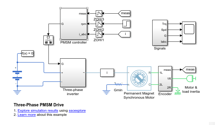
This example shows how to use the ee_solverUpdate function to configure the Solver Configuration and PMSM blocks in a model for simulation with the Partitioning solver and the Backward Euler solver. It also shows how to compare the simulation duration times and the results.

Open the model. At the MATLAB^® command prompt, enter this code.
See Code
openExample("simscapeelectrical/PMSMDriveExample") model = "PMSMDrive" open_system(model)
Two blocks that the ee_solverUpdate function can update are the Solver Configuration block and PMSM block.

Save the parameter settings for the two blocks.

See Code

The settings are saved to configBaseline array in the MATLAB workspace.

The settings of interest for the Solver Configuration block are:

Use local solver — The option to use a local Simscape solver is cleared.
Solver type — Backward Euler, a Simscape local fixed- cost solver, is specified. However, if you open the block dialog box, you can see that it is not enabled because the option to use a local solver is cleared.
Use fixed-cost runtime consistency iterations — The option to use fixed-cost is cleared. This option is also disabled when the option to use a local solver is cleared.

For the machine, the Zero sequence parameter is set to Include. Zero-sequence equations can cause numerical difficulty when you simulate with the Partitioning solver.

To return all simulation outputs within a single Simulink.SimulationOutput object so that you can later compare simulation times, enable the single-output format of the sim command.
```
% Enable single-output format 
set_param(model,'ReturnWorkspaceOutputs', 'on')
```

Mark the rotor torque signal, which connects the trqMotor From block to a Mux block, for Simulation Data Logging and viewing with the Simulation Data Inspector.

See Code

The logging badge marks the signal in the model.

Determine the results and how long it takes to simulate with the baseline settings.

See Code

Use ee_updateSolver function to change to the Backward Euler solver configuration. Save the configuration settings, and compare the settings to the baseline settings.

See Code

configDiff =

  1×1 cell array

    {'on'}

The option to use the local solver, which is set to Backward Euler by default, and the option to use fixed-cost runtime consistency iterations are now both selected.

Run a timed simulation using the Backward Euler solver.

See Code

If you change the local solver to the Partitioning solver and simulate the model now, an error occurs because of the zero-sequence terms. Use the ee_updateSolver function to configure the model for simulating with the Partitioning solver without generating an error. Save the configuration settings, compare the settings to baseline settings, and run a timed simulation.

See Code

configDiff =

  3×1 cell array

    {'NE_PARTITIONING_ADVANCER'         }
    {'ee.enum.park.zerosequence.exclude'}
    {'on'                               }

Warning: Initial conditions for nondifferential variables
not supported. The following states may deviate from
requested initial conditions:
   ['<a
   href="matlab:open_and_hilite_system('ee_pmsm_drive/Battery')"...
        >ee_pmsm_drive/Battery</a>']
   Battery.num_cycles
      o In ee.sources.battery_base
   ['<a
   href="matlab:open_and_hilite_system('ee_pmsm_drive/Permanent
   Magnet Synchronous Motor')">ee_pmsm_drive/Permanent
   Magnet Synchronous Motor</a>']
   Permanent_Magnet_Synchronous_Motor.angular_position

The solver type is now set to the Partitioning solver and the machine is configured to exclude zero-sequence terms.

The simulation runs without generating an error. It does generate a warning because initial conditions for nondifferential variables are not supported for the Partitioning solver.

Print tables that show:

Simulation time for each solver
Percent differences in speed for the local solvers versus the baseline global solver.

See Code

Simulation time on your machine may differ because simulation speed depends on machine processing power and the computational cost of concurrent processes. The local fixed-step Partitioning and Backward Euler solvers are faster than the baseline solver, which is a global, variable-step solver. The Partitioning solver is faster than the Backward Euler solver.

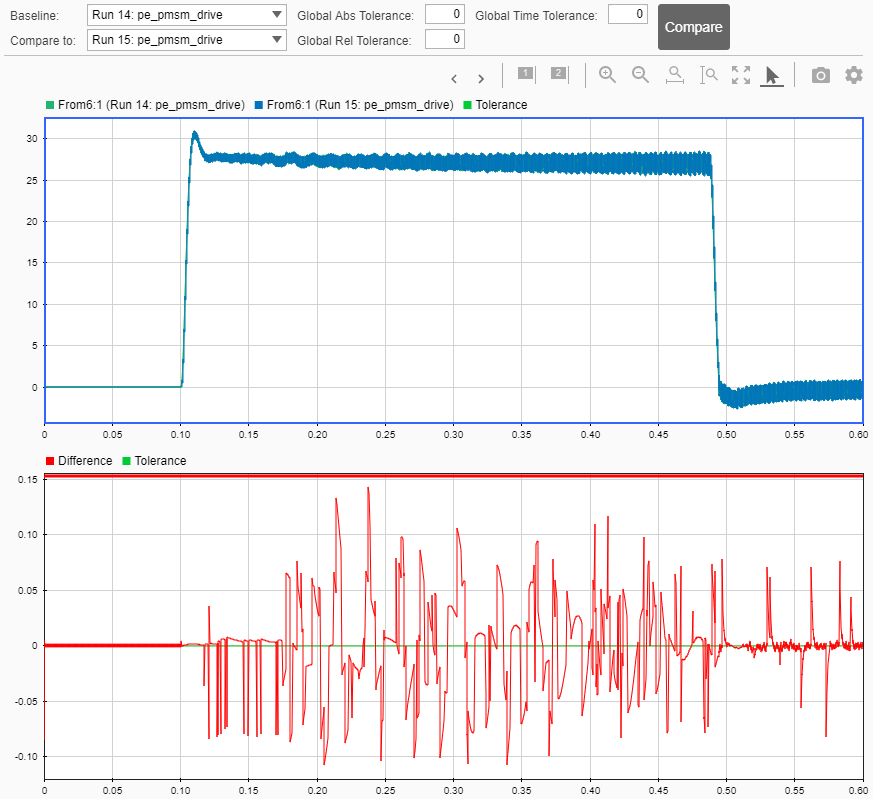
To compare the results, open the Simulation Data Inspector.
See Code
% Get Simulation Data Inspector run IDs for % the last three runs runIDs = Simulink.sdi.getAllRunIDs; runBackEuler = runIDs(end - 1); runPartition = runIDs(end); % Open the Simulation Data Inspector Simulink.sdi.view compBaselinePartition = Simulink.sdi.compareRuns(runBackEuler,... runPartition);
To see the comparison, click Compare and then click From6.

The first plot shows the overlay of the Backward Euler and Partitioning solver simulation results. The second plot shows how they differ. The default tolerance for differences is 0. To determine if the accuracy of the results meets your requirements, you can adjust the relative, absolute, and time tolerances. For more information, see Compare Simulation Data.

You can also use the ee_updateSolver function to reset the model for simulation with a global solver.

See Code

Limitations of the `ee_updateSolver` Function

Using the ee_updateSolver function does not guarantee that a simulation does not generate an error or that a simulation produces accurate results. To ensure that simulation accuracy meets your requirements, it is a recommended practice to compare simulation results to baseline results whenever you change model or block settings.