Cluster Data Using Gaussian Mixture Model
This topic provides an introduction to clustering with a Gaussian mixture model (GMM)
using the Statistics and Machine Learning Toolbox™ function cluster, and an example that shows the
effects of specifying optional parameters when fitting the GMM model using fitgmdist.
How Gaussian Mixture Models Cluster Data
Gaussian mixture models (GMMs) are often used for data clustering. You can use GMMs to perform either hard clustering or soft clustering on query data.
To perform hard clustering, the GMM assigns query data points
to the multivariate normal components that maximize the component posterior
probability, given the data. That is, given a fitted GMM, cluster assigns query data to the component yielding the highest posterior probability.
Hard clustering assigns a data point to exactly one cluster. For an example showing
how to fit a GMM to data, cluster using the fitted model, and estimate component
posterior probabilities, see Cluster Gaussian Mixture Data Using Hard Clustering.
Additionally, you can use a GMM to perform a more flexible clustering on data, referred to as soft (or fuzzy) clustering. Soft clustering methods assign a score to a data point for each cluster. The value of the score indicates the association strength of the data point to the cluster. As opposed to hard clustering methods, soft clustering methods are flexible because they can assign a data point to more than one cluster. When you perform GMM clustering, the score is the posterior probability. For an example of soft clustering with a GMM, see Cluster Gaussian Mixture Data Using Soft Clustering.
GMM clustering can accommodate clusters that have different sizes and correlation structures within them. Therefore, in certain applications,, GMM clustering can be more appropriate than methods such as k-means clustering. Like many clustering methods, GMM clustering requires you to specify the number of clusters before fitting the model. The number of clusters specifies the number of components in the GMM.
For GMMs, follow these best practices:
Consider the component covariance structure. You can specify diagonal or full covariance matrices, and whether all components have the same covariance matrix.
Specify initial conditions. The Expectation-Maximization (EM) algorithm fits the GMM. As in the k-means clustering algorithm, EM is sensitive to initial conditions and might converge to a local optimum. You can specify your own starting values for the parameters, specify initial cluster assignments for data points or let them be selected randomly, or specify use of the k-means++ algorithm.
Implement regularization. For example, if you have more predictors than data points, then you can regularize for estimation stability.
Fit GMM with Different Covariance Options and Initial Conditions
This example explores the effects of specifying different options for covariance structure and initial conditions when you perform GMM clustering.
Load Fisher's iris data set. Consider clustering the sepal measurements, and visualize the data in 2-D using the sepal measurements.
load fisheriris;
X = meas(:,1:2);
[n,p] = size(X);

plot(X(:,1),X(:,2),'.','MarkerSize',15);
title('Fisher''s Iris Data Set');
xlabel('Sepal length (cm)');
ylabel('Sepal width (cm)');

The number of components k in a GMM determines the number of subpopulations, or clusters. In this figure, it is difficult to determine if two, three, or perhaps more Gaussian components are appropriate. A GMM increases in complexity as k increases.
Specify Different Covariance Structure Options
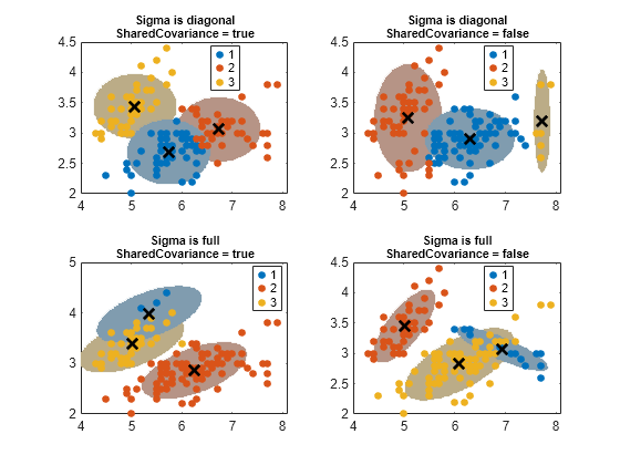
Each Gaussian component has a covariance matrix. Geometrically, the covariance structure determines the shape of a confidence ellipsoid drawn over a cluster. You can specify whether the covariance matrices for all components are diagonal or full, and whether all components have the same covariance matrix. Each combination of specifications determines the shape and orientation of the ellipsoids.
Specify three GMM components and 1000 maximum iterations for the EM algorithm. For reproducibility, set the random seed.
rng(3);
k = 3; % Number of GMM components
options = statset('MaxIter',1000);
Specify covariance structure options.
Sigma = {'diagonal','full'}; % Options for covariance matrix type
nSigma = numel(Sigma);

SharedCovariance = {true,false}; % Indicator for identical or nonidentical covariance matrices
SCtext = {'true','false'};
nSC = numel(SharedCovariance);
Create a 2-D grid covering the plane composed of extremes of the measurements. You will use this grid later to draw confidence ellipsoids over the clusters.
d = 500; % Grid length
x1 = linspace(min(X(:,1))-2, max(X(:,1))+2, d);
x2 = linspace(min(X(:,2))-2, max(X(:,2))+2, d);
[x1grid,x2grid] = meshgrid(x1,x2);
X0 = [x1grid(:) x2grid(:)];
Specify the following:
For all combinations of the covariance structure options, fit a GMM with three components.
Use the fitted GMM to cluster the 2-D grid.
Obtain the score that specifies a 95% probability threshold for each confidence region. This specification determines the length of the major and minor axes of the ellipsoids.
Color each ellipsoid using a similar color as its cluster.
threshold = sqrt(chi2inv(0.95,2));
count = 1;
for i = 1:nSigma
    for j = 1:nSC
        gmfit = fitgmdist(X,k,'CovarianceType',Sigma{i}, ...
            'SharedCovariance',SharedCovariance{j},'Options',options); % Fitted GMM
        clusterX = cluster(gmfit,X); % Cluster index
        mahalDist = sqrt(mahal(gmfit,X0)); % Distance from each grid point to each GMM component
        % Draw ellipsoids over each GMM component and show clustering result.
        subplot(2,2,count);
        h1 = gscatter(X(:,1),X(:,2),clusterX);
        hold on
            for m = 1:k
                idx = mahalDist(:,m)<=threshold;
                Color = h1(m).Color*0.75 - 0.5*(h1(m).Color - 1);
                h2 = plot(X0(idx,1),X0(idx,2),'.','Color',Color,'MarkerSize',1);
                uistack(h2,'bottom');
            end
        plot(gmfit.mu(:,1),gmfit.mu(:,2),'kx','LineWidth',2,'MarkerSize',10)
        title(sprintf('Sigma is %s\nSharedCovariance = %s',Sigma{i},SCtext{j}),'FontSize',8)
        legend(h1,{'1','2','3'})
        hold off
        count = count + 1;
    end
end

The probability threshold for the confidence region determines the length of the major and minor axes, and the covariance type determines the orientation of the axes. Note the following about options for the covariance matrices:
Diagonal covariance matrices indicate that the predictors are uncorrelated. The major and minor axes of the ellipses are parallel or perpendicular to the x and y axes. This specification increases the total number of parameters by , the number of predictors, for each component, but is more parsimonious than the full covariance specification.
Full covariance matrices allow for correlated predictors with no restriction to the orientation of the ellipses relative to the x and y axes. Each component increases the total number of parameters by , but captures the correlation structure among the predictors. This specification can cause overfitting.
Shared covariance matrices indicate that all components have the same covariance matrix. All ellipses are the same size and have the same orientation. This specification is more parsimonious than the unshared specification because the total number of parameters increases by the number of covariance parameters for one component only.
Unshared covariance matrices indicate that each component has its own covariance matrix. The size and orientation of all ellipses might differ. This specification increases the number of parameters by k times the number of covariance parameters for a component, but can capture covariance differences among components.
The figure also shows that cluster does not always preserve cluster order. If you cluster several fitted gmdistribution models, cluster can assign different cluster labels for similar components.
Specify Different Initial Conditions
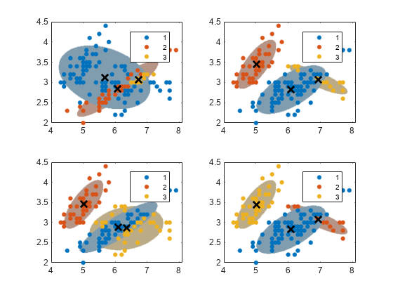
The algorithm that fits a GMM to the data can be sensitive to initial conditions. To illustrate this sensitivity, fit four different GMMs as follows:
For the first GMM, assign most data points to the first cluster.
For the second GMM, randomly assign data points to clusters.
For the third GMM, make another random assignment of data points to clusters.
For the fourth GMM, use k-means++ to obtain initial cluster centers.
initialCond1 = [ones(n-8,1); [2; 2; 2; 2]; [3; 3; 3; 3]]; % For the first GMM
initialCond2 = randsample(1:k,n,true); % For the second GMM
initialCond3 = randsample(1:k,n,true); % For the third GMM
initialCond4 = 'plus'; % For the fourth GMM
cluster0 = {initialCond1; initialCond2; initialCond3; initialCond4};
For all instances, use k = 3 components, unshared and full covariance matrices, the same initial mixture proportions, and the same initial covariance matrices. For stability when you try different sets of initial values, increase the number of EM algorithm iterations. Also, draw confidence ellipsoids over the clusters.
converged = nan(4,1);

for j = 1:4
    gmfit = fitgmdist(X,k,'CovarianceType','full', ...
        'SharedCovariance',false,'Start',cluster0{j}, ...
        'Options',options);
    clusterX = cluster(gmfit,X); % Cluster index
    mahalDist = sqrt(mahal(gmfit,X0)); % Distance from each grid point to each GMM component
    % Draw ellipsoids over each GMM component and show clustering result.
    subplot(2,2,j);
    h1 = gscatter(X(:,1),X(:,2),clusterX); % Distance from each grid point to each GMM component
    hold on;
    nK = numel(unique(clusterX));
    for m = 1:nK
        idx = mahalDist(:,m)<=threshold;
        Color = h1(m).Color*0.75 + -0.5*(h1(m).Color - 1);
        h2 = plot(X0(idx,1),X0(idx,2),'.','Color',Color,'MarkerSize',1);
        uistack(h2,'bottom');
    end
	plot(gmfit.mu(:,1),gmfit.mu(:,2),'kx','LineWidth',2,'MarkerSize',10)
    legend(h1,{'1','2','3'});
    hold off
    converged(j) = gmfit.Converged; % Indicator for convergence
end

sum(converged)
ans =
4
All algorithms converged. Each starting cluster assignment for the data points leads to a different, fitted cluster assignment. You can specify a positive integer for the name-value pair argument Replicates, which runs the algorithm the specified number of times. Subsequently, fitgmdist chooses the fit that yields the largest likelihood.
When to Regularize
Sometimes, during an iteration of the EM algorithm, a fitted covariance matrix can become ill conditioned, which means the likelihood is escaping to infinity. This problem can happen if one or more of the following conditions exist:
You have more predictors than data points.
You specify fitting with too many components.
Variables are highly correlated.
To overcome this problem, you can specify a small, positive number using the
'RegularizationValue' name-value pair argument.
fitgmdist adds this number to the diagonal elements of all
covariance matrices, which ensures that all matrices are positive definite.
Regularizing can reduce the maximal likelihood value.
Model Fit Statistics
In most applications, the number of components k and appropriate covariance structure Σ are unknown. One way you can tune a GMM is by comparing information criteria. Two popular information criteria are the Akaike Information Criterion (AIC) and Bayesian Information Criterion (BIC).
Both the AIC and BIC take the optimized, negative loglikelihood and then penalize
it with the number of parameters in the model (the model complexity). However, the
BIC penalizes for complexity more severely than the AIC. Therefore, the AIC tends to
choose more complex models that might overfit, and the BIC tends to choose simpler
models that might underfit. A good practice is to look at both criteria when
evaluating a model. Lower AIC or BIC values indicate better fitting models. Also,
ensure that your choices for k and the covariance matrix
structure are appropriate for your application. fitgmdist
stores the AIC and BIC of fitted gmdistribution model objects in
the properties AIC and
BIC.
You can access these properties by using dot notation. For an example showing how to
choose the appropriate parameters, see Tune Gaussian Mixture Models.
See Also
fitgmdist | gmdistribution | cluster
Topics
- Cluster Gaussian Mixture Data Using Hard Clustering
- Cluster Gaussian Mixture Data Using Soft Clustering
- Tune Gaussian Mixture Models
- Choose Cluster Analysis Method