Multivariate t Distribution

Definition

The probability density function of the d-dimensional multivariate Student's t distribution is given by

$f (x, Σ, ν) = \frac{1}{{| Σ |}^{1 / 2}} \frac{1}{\sqrt{{(ν π)}^{d}}} \frac{Γ ((ν + d) / 2)}{Γ (ν / 2)} {(1 + \frac{x^{'} Σ^{- 1} x}{ν})}^{- (ν + d) / 2} .$

where x is a 1-by-d vector, Σ is a d-by-d symmetric, positive definite matrix, and ν is a positive scalar. While it is possible to define the multivariate Student's t for singular Σ, the density cannot be written as above. For the singular case, only random number generation is supported. Note that while most textbooks define the multivariate Student's t with x oriented as a column vector, for the purposes of data analysis software, it is more convenient to orient x as a row vector, and Statistics and Machine Learning Toolbox™ software uses that orientation.

Background

The multivariate Student's t distribution is a generalization of the univariate Student's t to two or more variables. It is a distribution for random vectors of correlated variables, each element of which has a univariate Student's t distribution. In the same way as the univariate Student's t distribution can be constructed by dividing a standard univariate normal random variable by the square root of a univariate chi-square random variable, the multivariate Student's t distribution can be constructed by dividing a multivariate normal random vector having zero mean and unit variances by a univariate chi-square random variable.

The multivariate Student's t distribution is parameterized with a correlation matrix, Σ, and a positive scalar degrees of freedom parameter, ν. ν is analogous to the degrees of freedom parameter of a univariate Student's t distribution. The off-diagonal elements of Σ contain the correlations between variables. Note that when Σ is the identity matrix, variables are uncorrelated; however, they are not independent.

The multivariate Student's t distribution is often used as a substitute for the multivariate normal distribution in situations where it is known that the marginal distributions of the individual variables have fatter tails than the normal.

Example

Plot pdf and cdf of Multivariate t-Distribution

Open Live Script

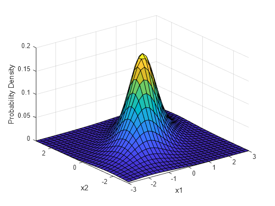
Plot the pdf of a bivariate Student's t distribution. You can use this distribution for a higher number of dimensions as well, although visualization is not easy.

Rho = [1 .6; .6 1];
nu = 5;
x1 = -3:.2:3; x2 = -3:.2:3;
[X1,X2] = meshgrid(x1,x2);
F = mvtpdf([X1(:) X2(:)],Rho,nu);
F = reshape(F,length(x2),length(x1));
surf(x1,x2,F);
axis([-3 3 -3 3 0 .2])
xlabel('x1'); ylabel('x2'); zlabel('Probability Density');

Figure contains an axes object. The axes object with xlabel x1, ylabel x2 contains an object of type surface.

Plot the cdf of a bivariate Student's t distribution.

F = mvtcdf([X1(:) X2(:)],Rho,nu);
F = reshape(F,length(x2),length(x1));
surf(x1,x2,F);
axis([-3 3 -3 3 0 1])
xlabel('x1'); ylabel('x2'); zlabel('Cumulative Probability');

Figure contains an axes object. The axes object with xlabel x1, ylabel x2 contains an object of type surface.

Since the bivariate Student's t distribution is defined on the plane, you can also compute cumulative probabilities over rectangular regions. For example, this contour plot illustrates the computation that follows, of the probability contained within the unit square shown in the figure.

contour(x1,x2,F,[.0001 .001 .01 .05:.1:.95 .99 .999 .9999]);
xlabel('x'); ylabel('y');
line([0 0 1 1 0],[1 0 0 1 1],'linestyle','--','color','k');

Figure contains an axes object. The axes object with xlabel x, ylabel y contains 2 objects of type contour, line.

Compute the value of the probability contained within the unit square.

F = mvtcdf([0 0],[1 1],Rho,nu)

F = 
0.1401

Computing a multivariate cumulative probability requires significantly more work than computing a univariate probability. By default, the mvtcdf function computes values to less than full machine precision and returns an estimate of the error, as an optional second output.

[F,err] = mvtcdf([0 0],[1 1],Rho,nu)

F = 
0.1401

err = 
1.0000e-08