Working with Probability Distributions
Probability distributions are theoretical distributions based on assumptions about a source population. The distributions assign probability to the event that a random variable has a specific, discrete value, or falls within a specified range of continuous values.
Statistics and Machine Learning Toolbox™ offers several ways to work with probability distributions.
Probability Distribution Objects — Create a probability distribution object by fitting a probability distribution to sample data or by specifying parameter values. Then, use object functions to evaluate the distribution, generate random numbers, and so on.
Apps and Interactive User Interfaces — Interactively fit and explore probability distributions by using the Distribution Fitter app, Probability Distribution Function Tool, and random number generation tool (
randtool)Distribution-Specific Functions and Generic Distribution Functions — These functions are useful for generating random numbers, computing summary statistics inside a loop or script, and passing a cdf or pdf as a function handle to another function. You can also use these functions to perform computations on arrays of parameter values rather than a single set of parameters.
For a list of distributions supported by Statistics and Machine Learning Toolbox, see Supported Distributions.
Probability Distribution Objects
Probability distribution objects allow you to fit a probability distribution to sample data, or define a distribution by specifying parameter values. You can then perform a variety of analyses on the distribution object.
Create Probability Distribution Objects
Estimate probability distribution parameters from sample data by fitting a
probability distribution object to the data using fitdist.
You can fit a single specified parametric or nonparametric distribution to the
sample data. You can also fit multiple distributions of the same type to the
sample data based on grouping variables. For most distributions,
fitdist uses maximum likelihood estimation (MLE) to
estimate the distribution parameters from the sample data. For more information
and additional syntax options, see fitdist.
Alternatively, you can create a probability distribution object with specified
parameter values using makedist.
Work with Probability Distribution Objects
Once you create a probability distribution object, you can use object functions to:
Compute confidence intervals for the distribution parameters (
paramci).Compute summary statistics, including mean (
mean), median (median), interquartile range (iqr), variance (var), and standard deviation (std).Evaluate the probability density function (
pdf).Evaluate the cumulative distribution function (
cdf) or the inverse cumulative distribution function (icdf).Compute the negative loglikelihood (
negloglik) and profile likelihood function (proflik) for the distribution.Generate random numbers from the distribution (
random).Truncate the distribution to specified lower and upper limits (
truncate).Plot the probability density function, cumulative distribution, or probability plot (
plot)
Save a Probability Distribution Object
To save your probability distribution object to a .MAT file:
In the toolbar, click Save Workspace. This option saves all of the variables in your workspace, including any probability distribution objects.
In the workspace browser, right-click the probability distribution object and select Save as. This option saves only the selected probability distribution object, not the other variables in your workspace.
Alternatively, you can save a probability distribution object directly from
the command line by using the save function.
save enables you to choose a file name and specify the
probability distribution object you want to save. If you do not specify an
object (or other variable), MATLAB® saves all of the variables in your workspace, including any
probability distribution objects, to the specified file name. For more
information and additional syntax options, see save.
Analyze Distribution Using Probability Distribution Objects
This example shows how to use probability distribution objects to perform a multistep analysis on a fitted distribution.
The analysis illustrates how to:
Fit a probability distribution to sample data that contains exam grades of 120 students by using
fitdist.Compute the mean of the exam grades by using
mean.Plot a histogram of the exam grade data, overlaid with a plot of the pdf of the fitted distribution, by using
plotandpdf.Compute the boundary for the top 10 percent of student grades by using
icdf.Save the fitted probability distribution object by using
save.
Load the sample data.
load examgradesThe sample data contains a 120-by-5 matrix of exam grades. The exams are scored on a scale of 0 to 100.
Create a vector containing the first column of exam grade data.
x = grades(:,1);
Fit a normal distribution to the sample data by using fitdist to create a probability distribution object.
pd = fitdist(x,'Normal')pd =
NormalDistribution
Normal distribution
mu = 75.0083 [73.4321, 76.5846]
sigma = 8.7202 [7.7391, 9.98843]
fitdist returns a probability distribution object, pd, of the type NormalDistribution. This object contains the estimated parameter values, mu and sigma, for the fitted normal distribution. The intervals next to the parameter estimates are the 95% confidence intervals for the distribution parameters.
Compute the mean of the students' exam grades using the fitted distribution object, pd.
m = mean(pd)
m =
75.0083
The mean of the exam grades is equal to the mu parameter estimated by fitdist.
Plot a histogram of the exam grades. Overlay a plot of the fitted pdf to visually compare the fitted normal distribution with the actual exam grades.
x_pdf = [1:0.1:100];
y = pdf(pd,x_pdf);

figure
histogram(x,'Normalization','pdf')
line(x_pdf,y)
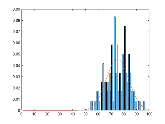
The pdf of the fitted distribution follows the same shape as the histogram of the exam grades.
Determine the boundary for the upper 10 percent of student exam grades by using the inverse cumulative distribution function (icdf). This boundary is equivalent to the value at which the cdf of the probability distribution is equal to 0.9. In other words, 90 percent of the exam grades are less than or equal to the boundary value.
A = icdf(pd,0.9)
A =
86.1837
Based on the fitted distribution, 10 percent of students received an exam grade greater than 86.1837. Equivalently, 90 percent of students received an exam grade less than or equal to 86.1837.
Save the fitted probability distribution, pd, as a file named myobject.mat.
save('myobject.mat','pd')
Apps and Interactive User Interfaces
Apps and user interfaces provide an interactive approach to working with parametric and nonparametric probability distributions.
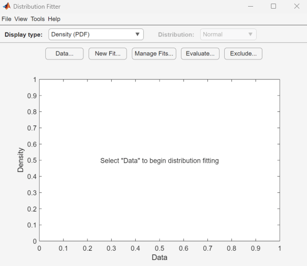
Use the Distribution Fitter app to interactively fit a distribution to sample data, and export a probability distribution object to the workspace.
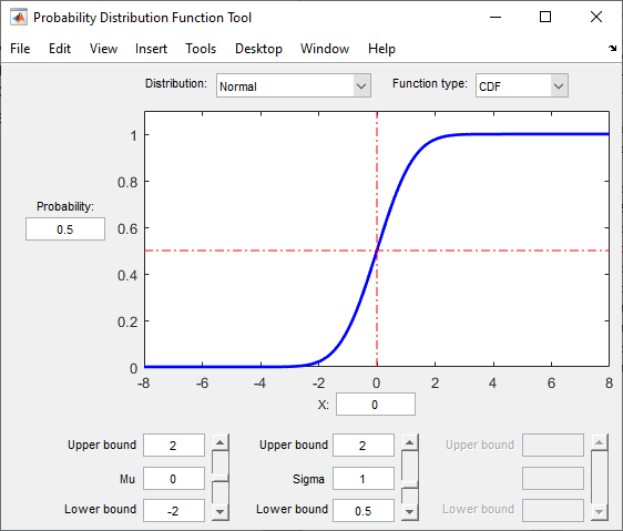
Use the Probability Distribution Function Tool to visually explore the effect on the pdf and cdf of changing the distribution parameter values.
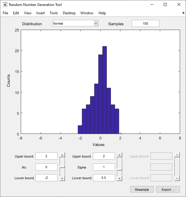
Use the Random Number Generation user interface (
randtool) to interactively generate random numbers from a probability distribution with specified parameter values and export them to the workspace.
Distribution Fitter App
The Distribution Fitter app allows you to interactively fit a probability distribution to your data. You can display different types of plots, compute confidence bounds, and evaluate the fit of the data. You can also exclude data from the fit. You can save the data, and export the fit to your workspace as a probability distribution object to perform further analysis.
Load the Distribution Fitter app from the Apps tab, or by entering
distributionFitter in the command window. For more
information, see Model Data Using the Distribution Fitter App.
Probability Distribution Function Tool
The Probability Distribution Function Tool
visually explores probability distributions. You can load the Probability
Distribution Function user interface by entering disttool in
the command window.
Random Number Generation Tool
The Random Number Generation user interface generates random data from a specified distribution and exports the results to your workspace. You can use this tool to explore the effects of changing parameters and sample size on the distributions.
The Random Number Generation user interface allows you to set parameter values for the distribution and change their lower and upper bounds; draw another sample from the same distribution, using the same size and parameters; and export the current random sample to your workspace for use in further analysis. A dialog box enables you to provide a name for the sample.
Distribution-Specific Functions and Generic Distribution Functions
Using distribution-specific functions and generic distribution functions is useful for generating random numbers, computing summary statistics inside a loop or script, and passing a cdf or pdf as a function handle to another function. You can also use these functions to perform computations on arrays of parameter values rather than a single set of parameters.
Distribution-specific functions — Some of the supported distributions have distribution-specific functions. These functions use the following abbreviations, as in
normpdf,normcdf,norminv,normstat,normfit,normlike, andnormrnd:pdf— Probability density functionscdf— Cumulative distribution functionsinv— Inverse cumulative distribution functionsstat— Distribution statistics functionsfit— Distribution Fitter functionslike— Negative loglikelihood functionsrnd— Random number generators
Generic distribution functions — Use
cdf,icdf,mle,pdf, andrandomwith a specified distribution name and parameters.
Analyze Distribution Using Distribution-Specific Functions
This example shows how to use distribution-specific functions to perform a multistep analysis on a fitted distribution.
The analysis illustrates how to:
Fit a probability distribution to sample data that contains exam grades of 120 students by using
normfit.Plot a histogram of the exam grade data, overlaid with a plot of the pdf of the fitted distribution, by using
plotandnormpdf.Compute the boundary for the top 10 percent of student grades by using
norminv.Save the estimated distribution parameters by using
save.
You can perform the same analysis using a probability distribution object. See Analyze Distribution Using Probability Distribution Objects.
Load the sample data.
load examgradesThe sample data contains a 120-by-5 matrix of exam grades. The exams are scored on a scale of 0 to 100.
Create a vector containing the first column of exam grade data.
x = grades(:,1);
Fit a normal distribution to the sample data by using normfit.
[mu,sigma,muCI,sigmaCI] = normfit(x)
mu =
75.0083
sigma =
8.7202
muCI = 2×1

   73.4321
   76.5846
sigmaCI = 2×1

    7.7391
    9.9884
The normfit function returns the estimates of normal distribution parameters and the 95% confidence intervals for the parameter estimates.
Plot a histogram of the exam grades. Overlay a plot of the fitted pdf to visually compare the fitted normal distribution with the actual exam grades.
x_pdf = [1:0.1:100];
y = normpdf(x_pdf,mu,sigma);

figure
histogram(x,'Normalization','pdf')
line(x_pdf,y)

The pdf of the fitted distribution follows the same shape as the histogram of the exam grades.
Determine the boundary for the upper 10 percent of student exam grades by using the normal inverse cumulative distribution function. This boundary is equivalent to the value at which the cdf of the probability distribution is equal to 0.9. In other words, 90 percent of the exam grades are less than or equal to the boundary value.
A = norminv(0.9,mu,sigma)
A =
86.1837
Based on the fitted distribution, 10 percent of students received an exam grade greater than 86.1837. Equivalently, 90 percent of students received an exam grade less than or equal to 86.1837.
Save the estimated distribution parameters as a file named myparameter.mat.
save('myparameter.mat','mu','sigma')
Use Probability Distribution Functions as Function Handle
This example shows how to use the probability distribution function normcdf as a function handle in the chi-square goodness of fit test (chi2gof).
This example tests the null hypothesis that the sample data contained in the input vector, x, comes from a normal distribution with parameters µ and σ equal to the mean (mean) and standard deviation (std) of the sample data, respectively.
rng('default') % For reproducibility
x = normrnd(50,5,100,1);
h = chi2gof(x,'cdf',{@normcdf,mean(x),std(x)})
h =
0
The returned result h = 0 indicates that chi2gof does not reject the null hypothesis at the default 5% significance level.
This next example illustrates how to use probability distribution functions as a function handle in the slice sampler (slicesample). The example uses normpdf to generate a random sample of 2,000 values from a standard normal distribution, and plots a histogram of the resulting values.
rng('default') % For reproducibility
x = slicesample(1,2000,'pdf',@normpdf,'thin',5,'burnin',1000);
histogram(x)
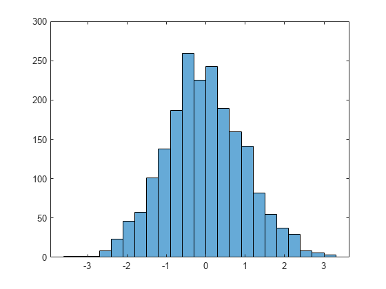
The histogram shows that, when using normpdf, the resulting random sample has a standard normal distribution.
If you pass the probability distribution function for the exponential distribution pdf (exppdf) as a function handle instead of normpdf, then slicesample generates the 2,000 random samples from an exponential distribution with a default parameter value of µ equal to 1.
rng('default') % For reproducibility
x = slicesample(1,2000,'pdf',@exppdf,'thin',5,'burnin',1000);
histogram(x)
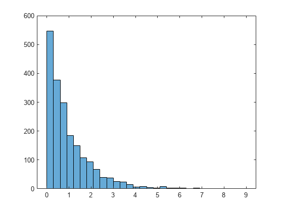
The histogram shows that the resulting random sample when using exppdf has an exponential distribution.
See Also
fitdist | makedist | randtool | Distribution Fitter | Probability Distribution Function Tool