Model Data Using the Distribution Fitter App
The Distribution Fitter app provides a visual, interactive approach to fitting univariate distributions to data.
Explore Probability Distributions Interactively
You can use the Distribution Fitter app to interactively fit probability distributions to data imported from the MATLAB® workspace. You can choose from 22 built-in probability distributions, or create your own custom distribution. The app displays the fitted distribution over plots of the empirical distributions, including pdf, cdf, probability plots, and survivor functions. You can export the fit data, including fitted parameter values, to the workspace for further analysis.
Distribution Fitter App Workflow
To fit a probability distribution to your sample data:
On the MATLAB Toolstrip, click the Apps tab. In the Math, Statistics and Optimization group, open the Distribution Fitter app. Alternatively, at the command prompt, enter
distributionFitter.Import your sample data, or create a data vector directly in the app. You can also manage your data sets and choose which one to fit. See Create and Manage Data Sets.
Create a new fit for your data. See Create a New Fit.
Display the results of the fit. You can choose to display the density (pdf), cumulative probability (cdf), quantile (inverse cdf), probability plot (choose one of several distributions), survivor function, and cumulative hazard. See Display Results.
You can create additional fits, and manage multiple fits from within the app. See Manage Fits.
Evaluate probability functions for the fit. You can choose to evaluate the density (pdf), cumulative probability (cdf), quantile (inverse cdf), survivor function, and cumulative hazard. See Evaluate Fits.
Improve the fit by excluding certain data. You can specify bounds for the data to exclude, or you can exclude data graphically using a plot of the values in the sample data. See Exclude Data.
Save your current Distribution Fitter app session so you can open it later. See Save and Load Sessions.
Create and Manage Data Sets
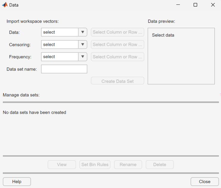
To open the Data dialog box, click the Data button in the Distribution Fitter app.
Import Data
Create a data set by importing a vector from the MATLAB workspace using the Import workspace vectors options.
Data — In the Data field, the drop-down list contains the names of all matrices and vectors, other than 1-by-1 matrices (scalars) in the MATLAB workspace. Select the array containing the data that you want to fit. The actual data you import must be a vector. If you select a matrix in the Data field, the first column of the matrix is imported by default. To select a different column or row of the matrix, click Select Column or Row. The matrix appears in the Select Column or Row dialog box. You can select a row or column by highlighting it.
Alternatively, you can enter any valid MATLAB expression in the Data field.
When you select a vector in the Data field, a histogram of the data appears in the Data preview pane.
Censoring — If some of the points in the data set are censored, enter a Boolean vector of the same size as the data vector, specifying the censored entries of the data. A
1in the censoring vector specifies that the corresponding entry of the data vector is censored. A0specifies that the entry is not censored. If you enter a matrix, you can select a column or row by clicking Select Column or Row. If you do not have censored data, leave the Censoring field blank.Frequency — Enter a vector of positive integers of the same size as the data vector to specify the frequency of the corresponding entries of the data vector. For example, a value of
7in the 15th entry of frequency vector specifies that there are 7 data points corresponding to the value in the 15th entry of the data vector. If all entries of the data vector have frequency 1, leave the Frequency field blank.Data set name — Enter a name for the data set that you import from the workspace, such as
My
data
.
After you have entered the information in the preceding fields,
click Create Data Set to create the data set My
data.
Manage Data Sets
View and manage the data sets that you create using the Manage data
sets pane. When you create a data set, its name appears in the
Data set list. The following figure shows the
Manage data sets pane after creating the data set
My data.
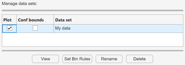
For each data set in the Data set list, you can:
Select the Plot check box to display a plot of the data in the main Distribution Fitter app window. When you create a new data set, Plot is selected by default. Clearing the Plot check box removes the data from the plot in the main window. You can specify the type of plot displayed in the Display type field in the main window.
If Plot is selected, you can also select Conf bounds to display confidence interval bounds for the plot in the main window. These bounds are pointwise confidence bounds around the empirical estimates of these functions. The bounds are displayed only when you set Display Type in the main window to one of the following:
Cumulative probability (CDF)Survivor functionCumulative hazard
The Distribution Fitter app cannot display confidence bounds on density
(PDF), quantile (inverse
CDF), or probability plots. Clearing the Conf
bounds check box removes the confidence bounds from the plot in
the main window.
When you select a data set from the list, you can access the following buttons:
View — Display the data in a table in a new window.
Set Bin Rules — Defines the histogram bins used in a density (PDF) plot.
Rename — Rename the data set.
Delete — Delete the data set.
Set Bin Rules
To set bin rules for the histogram of a data set, click Set Bin Rules to open the Set Bin Rules dialog box.

You can select from the following rules:
Freedman-Diaconis rule — Algorithm that chooses bin widths and locations automatically, based on the sample size and the spread of the data. This rule is the default for all data, except data that consists of integers only.
Scott rule — Algorithm intended for data that are approximately normal. The algorithm chooses bin widths and locations automatically.
Number of bins — Enter the number of bins. All bins have equal widths.
Bins centered on integers — Specifies bins centered on integers. This is the default rule for data that consists of integers only.
Bin width — Enter the width of each bin. If you select this option, you can also select:
Automatic bin placement — Place the edges of the bins at integer multiples of the Bin width.
Bin boundary at — Enter a scalar to specify the boundaries of the bins. The boundary of each bin is equal to this scalar plus an integer multiple of the Bin width.
You can also:
Apply to all existing data sets — Apply the rule to all data sets. Otherwise, the rule is applied only to the data set currently selected in the Data dialog box.
Save as default — Apply the current rule to any new data sets that you create. You can set default bin width rules by selecting Set Default Bin Rules from the Tools menu in the main window.
Set Default Bin Rules
To set default bin rules for all histograms created in the app, select Set Default Bin Rules from the Tools menu in the main window. The Set Default Bin Rules dialog box opens.


The dialog box contains an additional option for setting the rule as Automatic. When this option is selected, the default bin rule for data that consists of only integers is Bins centered on integers, and the default bin rule for all other types of data is the Freedman-Diaconis rule.
Create a New Fit
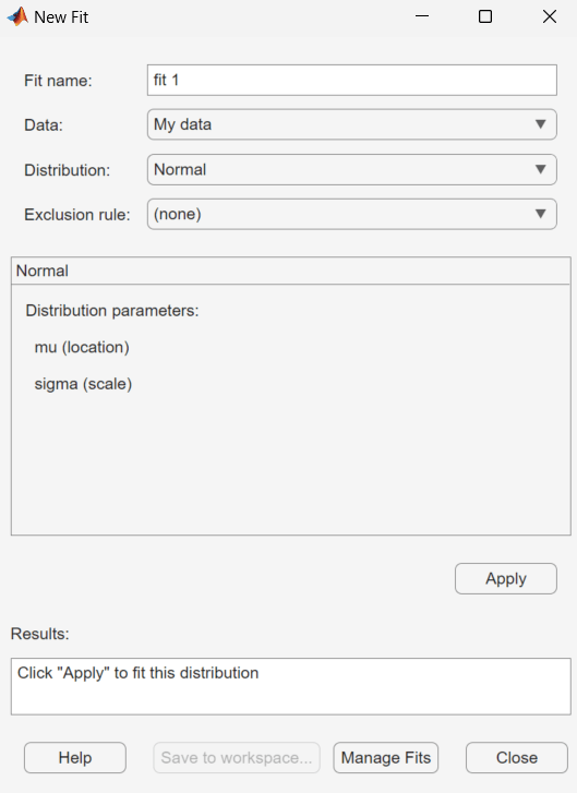
Click the New Fit button at the top of
the main window to open the New Fit dialog box. If you created the
data set My data, it appears in the Data field.
| Field Name | Description |
|---|---|
| Fit Name | Enter a name for the fit. |
| Data | Select the data set to which you want to fit a distribution from the drop-down list. |
| Distribution | Select the type of distribution to fit from the Distribution drop-down list. Only the distributions that apply to the values of the selected data set appear in the Distribution field. For example, when the data include values that are zero or negative, positive distributions are not displayed. You can specify either a parametric or a nonparametric distribution. When you select a parametric distribution from the drop-down list, a description of its parameters appears. Distribution Fitter estimates these parameters to fit the distribution to the data set. If you select the binomial distribution or the generalized extreme value distribution, you must specify a fixed value for one of the parameters. The pane contains a text field into which you can specify that parameter. When you select
|
| Exclusion rule | Specify a rule to exclude some data. Create an exclusion rule by clicking Exclude in the Distribution Fitter app. For more information, see Exclude Data. |
Apply the New Fit
Click Apply to fit the distribution. For a parametric fit, the Results pane displays the values of the estimated parameters. For a nonparametric fit, the Results pane displays information about the fit.
When you click Apply, the Distribution Fitter app displays a plot of the distribution and the corresponding data.
Note
When you click Apply, the title of the dialog box changes to Edit Fit. You can now make changes to the fit you just created and click Apply again to save them. After closing the Edit Fit dialog box, you can reopen it from the Fit Manager dialog box at any time to edit the fit.
After applying the fit, you can save the information to the workspace using probability distribution objects by clicking Save to workspace.
Available Distributions
All of the distributions available in the Distribution Fitter
app are supported elsewhere in Statistics and Machine Learning Toolbox™ software. You
can use the fitdist function
to fit any of the distributions supported by the app. Many distributions
also have dedicated fitting functions. These functions compute the
majority of the fits in the Distribution Fitter app, and are referenced
in the following list. Other fits are computed using functions internal
to the Distribution Fitter app.
Not all of the distributions listed are available for all data sets. The Distribution Fitter app determines the extent of the data (nonnegative, unit interval, and so on) and displays appropriate distributions in the Distribution drop-down list. Distribution data ranges are given parenthetically in the following list.
Beta (unit interval values) distribution, fit using the function
betafit.Binomial (nonnegative integer values) distribution, fit using the function
binopdf.Birnbaum-Saunders (positive values) distribution.
Burr Type XII (positive values) distribution.
Exponential (nonnegative values) distribution, fit using the function
expfit.Extreme value (all values) distribution, fit using the function
evfit.Gamma (positive values) distribution, fit using the function
gamfit.Generalized extreme value (all values) distribution, fit using the function
gevfit.Generalized Pareto (all values) distribution, fit using the function
gpfit.Inverse Gaussian (positive values) distribution.
Logistic (all values) distribution.
Loglogistic (positive values) distribution.
Lognormal (positive values) distribution, fit using the function
lognfit.Nakagami (positive values) distribution.
Negative binomial (nonnegative integer values) distribution, fit using the function
nbinpdf.Nonparametric (all values) distribution, fit using the function
ksdensity.Normal (all values) distribution, fit using the function
normfit.Poisson (nonnegative integer values) distribution, fit using the function
poisspdf.Rayleigh (positive values) distribution using the function
raylfit.Rician (positive values) distribution.
t location-scale (all values) distribution.
Weibull (positive values) distribution using the function
wblfit.
Further Options for Nonparametric Fits
When you select Non-parametric in
the Distribution field, a set of options
appears in the Non-parametric pane, as shown
in the following figure.
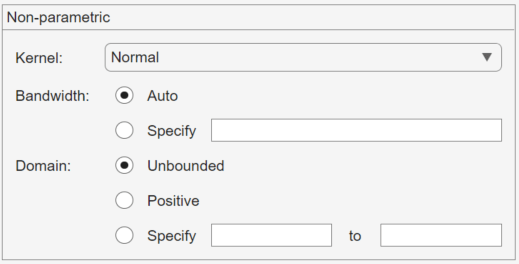
The options for nonparametric distributions are:
Kernel — Type of kernel function to use.
NormalBoxTriangleEpanechnikov
Bandwidth — The bandwidth of the kernel smoothing window. Select Auto for a default value that is optimal for estimating normal densities. After you click Apply, this value appears in the Results pane. Select Specify and enter a smaller value to reveal features such as multiple modes or a larger value to make the fit smoother.
Domain — The allowed x-values for the density.
Unbounded — The density extends over the whole real line.
Positive — The density is restricted to positive values.
Specify — Enter lower and upper bounds for the domain of the density.
When you select Positive or Specify, the nonparametric fit has zero probability outside the specified domain.
Display Results
The Distribution Fitter app window displays plots of:
The data sets for which you select Plot in the Data dialog box.
The fits for which you select Plot in the Fit Manager dialog box.
Confidence bounds for:
The data sets for which you select Conf bounds in the Data dialog box.
The fits for which you select Conf bounds in the Fit Manager dialog box.
The following fields are available.
Display Type
Specify the type of plot to display using the Display Type field in the main app window. Each type corresponds to a probability function, for example, a probability density function. You can choose from the following display types:
Density (PDF)— Display a probability density function (PDF) plot for the fitted distribution. The main window displays data sets using a probability histogram, in which the height of each rectangle is the fraction of data points that lie in the bin divided by the width of the bin. This makes the sum of the areas of the rectangles equal to 1.Cumulative probability (CDF)— Display a cumulative probability plot of the data. The main window displays data sets using a cumulative probability step function. The height of each step is the cumulative sum of the heights of the rectangles in the probability histogram.Quantile (inverse CDF)— Display a quantile (inverse CDF) plot.Probability plot— Display a probability plot of the data. Specify the type of distribution used to construct the probability plot in the Distribution field. This field is only available when you selectProbability plot. The choices for the distribution are:ExponentialExtreme ValueHalf NormalLog-LogisticLogisticLognormalNormalRayleighWeibull
You can also create a probability plot against a parametric fit that you create in the New Fit dialog box. When you create these fits, they are added at the bottom of the Distribution drop-down list.
Survivor function— Display survivor function plot of the data.Cumulative hazard— Display cumulative hazard plot of the data.Note
If the plotted data includes
0or negative values, some distributions are unavailable.
Confidence Bounds
You can display confidence bounds for data sets and fits when
you set Display Type to Cumulative
probability (CDF), Survivor function, Cumulative
hazard, or, for fits only, Quantile (inverse
CDF).
To display bounds for a data set, select Conf bounds next to the data set in the Manage data sets pane of the Data dialog box.
To display bounds for a fit, select Conf bounds next to the fit in the Fit Manager dialog box. Confidence bounds are not available for all fit types.
To set the confidence level for the bounds, select Confidence
Level from the View menu
in the main window and choose from the options.
Manage Fits
Click the Manage Fits button to open the Fit Manager dialog box.

The Table of fits displays a list of the fits that you create, with the following options:
Plot — Displays a plot of the fit in the main window of the Distribution Fitter app. When you create a new fit, Plot is selected by default. Clearing the Plot check box removes the fit from the plot in the main window.
Conf bounds — If you select Plot, you can also select Conf bounds to display confidence bounds in the plot. The bounds are displayed when you set Display type in the main window to one of the following:
Cumulative probability (CDF)Quantile (inverse CDF)Survivor functionCumulative hazard
The Distribution Fitter app cannot display confidence bounds on density (
PDF) or probability plots. Bounds are not supported for nonparametric fits and some parametric fits.Clearing the Conf bounds check box removes the confidence intervals from the plot in the main window.
When you select a fit in the Table of fits, the following buttons are enabled below the table:
New Fit — Open a New Fit window.
Copy — Create a copy of the selected fit.
Edit — Open an Edit Fit dialog box, to edit the fit.
Note
You can edit only the currently selected fit in the Edit Fit dialog box. To edit a different fit, select it in the Table of fits and click Edit to open another Edit Fit dialog box.
Save to workspace — Save the selected fit as a distribution object.
Delete — Delete the selected fit.
Evaluate Fits
Use the Evaluate dialog box to evaluate your fitted distribution at any data points you choose. To open the dialog box, click the Evaluate button.
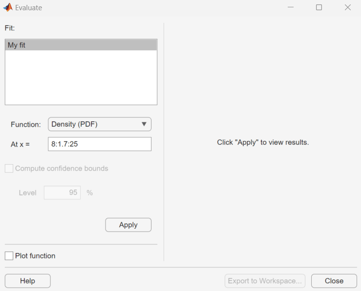
In the Evaluate dialog box, choose from the following items:
Fit pane — Display the names of existing fits. Select one or more fits that you want to evaluate. Using your platform specific functionality, you can select multiple fits.
Function — Select the type of probability function that you want to evaluate for the fit. The available functions are:
Density (PDF)— Computes a probability density function.Cumulative probability (CDF)— Computes a cumulative probability function.Quantile (inverse CDF)— Computes a quantile (inverse CDF) function.Survivor function— Computes a survivor function.Cumulative hazard— Computes a cumulative hazard function.Hazard rate— Computes the hazard rate.
At x = — Enter a vector of points or the name of a workspace variable containing a vector of points at which you want to evaluate the distribution function. If you change Function to
Quantile (inverse CDF), the field name changes to At p =, and you enter a vector of probability values.Compute confidence bounds — Select this box to compute confidence bounds for the selected fits. The check box is enabled only if you set Function to one of the following:
Cumulative probability (CDF)Quantile (inverse CDF)Survivor functionCumulative hazard
The Distribution Fitter app cannot compute confidence bounds for nonparametric fits and for some parametric fits. In these cases, it returns
NaNfor the bounds.Level — Set the level for the confidence bounds.
Plot function — Select this box to display a plot of the distribution function, evaluated at the points you enter in the At x = field, in a new window.
Note
The settings for Compute confidence bounds, Level, and Plot function do not affect the plots that are displayed in the main window of the Distribution Fitter app. The settings apply only to plots you create by clicking Plot function in the Evaluate window.
To apply these evaluation settings to the selected fit, click Apply.
The following figure shows the results of evaluating the cumulative distribution
function for the fit My fit, at the points in the vector
8:1.7:25.

The columns of the table to the right of the Fit pane display the following values:
X — The entries of the vector that you enter in At x = field.
F(X) — The corresponding values of the CDF at the entries of X.
LB — The lower bounds for the confidence interval, if you select Compute confidence bounds.
UB — The upper bounds for the confidence interval, if you select Compute confidence bounds.
To save the data displayed in the table to a matrix in the MATLAB workspace, click Export to Workspace.
Exclude Data
To exclude values from fit, open the Exclude window by clicking the Exclude button. In the Exclude window, you can create rules for excluding specified data values. When you create a new fit in the New Fit window, you can use these rules to exclude data from the fit.

To create an exclusion rule:
Exclusion Rule Name — Enter a name for the exclusion rule.
Exclude Sections — Specify bounds for the excluded data:
In the Lower limit: exclude data drop-down list, select
<=or<and enter a scalar value in the field to the right. Depending on which operator you select, the app excludes from the fit any data values that are less than or equal to the scalar value, or less than the scalar value, respectively.In the Upper limit: exclude data drop-down list, select
>=or>and enter a scalar value in the field to the right. Depending on which operator you select, the app excludes from the fit any data values that are greater than or equal to the scalar value, or greater than the scalar value, respectively.
OR
Click the Exclude Graphically button to define the exclusion rule by displaying a plot of the values in a data set and selecting the bounds for the excluded data. For example, if you created the data set
My dataas described in Create and Manage Data Sets, select it from the Select data drop-down list, and then click the Exclude Graphically button. The app displays the values inMy datain a new window.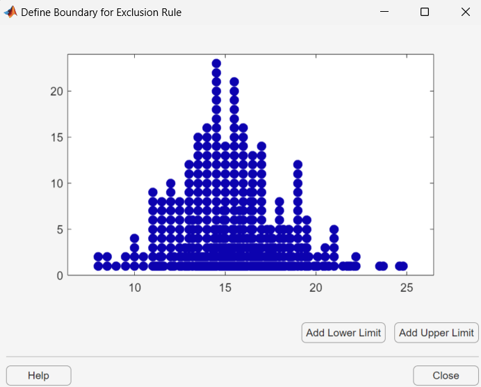
To set a lower limit for the boundary of the excluded region, click Add Lower Limit. The app displays a vertical line on the left side of the plot window. Move the line to the point you where you want the lower limit, as shown in the following figure.

Move the vertical line to change the value displayed in the Lower limit: exclude data field in the Exclude window.

The value displayed corresponds to the x-coordinate of the vertical line.
Similarly, you can set the upper limit for the boundary of the excluded region by clicking Add Upper Limit, and then moving the vertical line that appears at the right side of the plot window. After setting the lower and upper limits, click Close and return to the Exclude window.
Create Exclusion Rule — Once you have set the lower and upper limits for the boundary of the excluded data, click Create Exclusion Rule to create the new rule. The name of the new rule appears in the Existing exclusion rules pane.
Selecting an exclusion rule in the Existing exclusion rules pane enables the following buttons:
Copy — Creates a copy of the rule, which you can then modify. To save the modified rule under a different name, click Create Exclusion Rule.
View — Opens a new window in which you can see the data points excluded by the rule. The following figure shows a typical example.
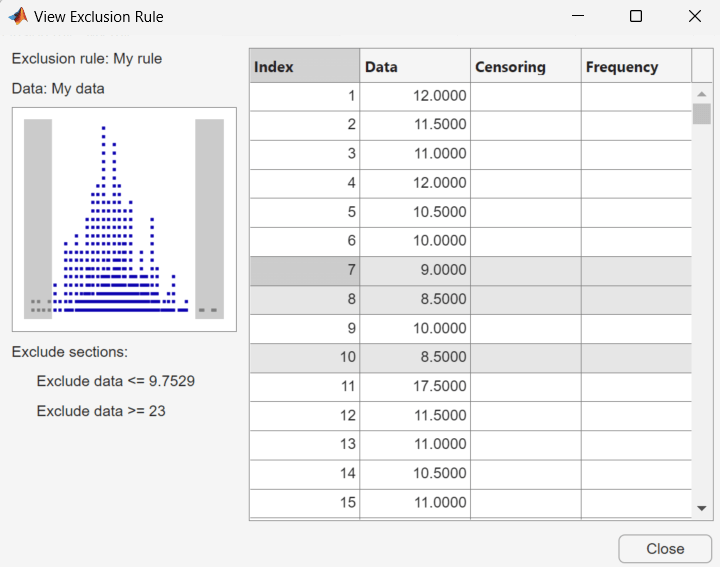
The shaded areas in the plot graphically display which data points are excluded. The table to the right lists all data points. The shaded rows indicate excluded points.
Rename — Rename the rule.
Delete — Delete the rule.
After you define an exclusion rule, you can use it when you fit a distribution to your data. The rule does not exclude points from the display of the data set.
Save and Load Sessions
Save your work in the current session, and then load it in a subsequent session, so that you can continue working where you left off.
Save a Session
To save the current session, from the File menu in the main window,
select Save Session. A dialog box opens and prompts
you to enter a file name, for example my_session.dfit. Click
Save to save the following items created in the
current session:
Data sets
Fits
Exclusion rules
Plot settings
Bin width rules
Load a Session
To load a previously saved session, from the File menu
in the main window, select Load Session.
Enter the name of a previously saved session. Click Open to
restore the information from the saved session to the current session.
Generate a File to Fit and Plot Distributions
Use the Generate Code option in the File
menu to create a file that:
Fits the distributions in the current session to any data vector in the MATLAB workspace.
Plots the data and the fits.
After you end the current session, you can use the file to create plots in a standard MATLAB figure window, without reopening the Distribution Fitter app.
As an example, if you created the fit described in Create a New Fit, do the following steps:
From the File menu, select
Generate Code.In the MATLAB Editor window, choose File > Save as. Save the file as
normal_fit.min a folder on the MATLAB path.
You can then apply the function normal_fit to
any vector of data in the MATLAB workspace. For example, the
following commands:
new_data = normrnd(4.1, 12.5, 100, 1);
newfit = normal_fit(new_data)
legend('New Data', 'My fit')
generate newfit, a fitted normal distribution
of the data. The commands also generate a plot of the data and the
fit.
newfit =

  NormalDistribution

  Normal distribution
       mu = 5.63857   [2.7555, 8.52163]
    sigma =   14.53   [12.7574, 16.8791]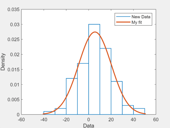
Note
By default, the file labels the data in the legend using the
same name as the data set in the Distribution Fitter app. You can
change the label using the legend command, as illustrated
by the preceding example.