Overview

A kernel distribution is a nonparametric representation of the probability density function (pdf) of a random variable. You can use a kernel distribution when a parametric distribution cannot properly describe the data, or when you want to avoid making assumptions about the distribution of the data. A kernel distribution is defined by a smoothing function and a bandwidth value, which control the smoothness of the resulting density curve.

Kernel Density Estimator

The kernel density estimator is the estimated pdf of a random variable. For any real values of x, the kernel density estimator's formula is given by

where x₁, x₂, …, x_n are random samples from an unknown distribution, n is the sample size, $$K(·)$$ is the kernel smoothing function, and h is the bandwidth.

Kernel Smoothing Function

The kernel smoothing function defines the shape of the curve used to generate the pdf. Similar to a histogram, the kernel distribution builds a function to represent the probability distribution using the sample data. But unlike a histogram, which places the values into discrete bins, a kernel distribution sums the component smoothing functions for each data value to produce a smooth, continuous probability curve. The following plots show a visual comparison of a histogram and a kernel distribution generated from the same sample data.

A histogram represents the probability distribution by establishing bins and placing each data value in the appropriate bin.

SixMPG = [13;15;23;29;32;34];
figure
histogram(SixMPG)

Because of this bin count approach, the histogram produces a discrete probability density function. This might be unsuitable for certain applications, such as generating random numbers from a fitted distribution.

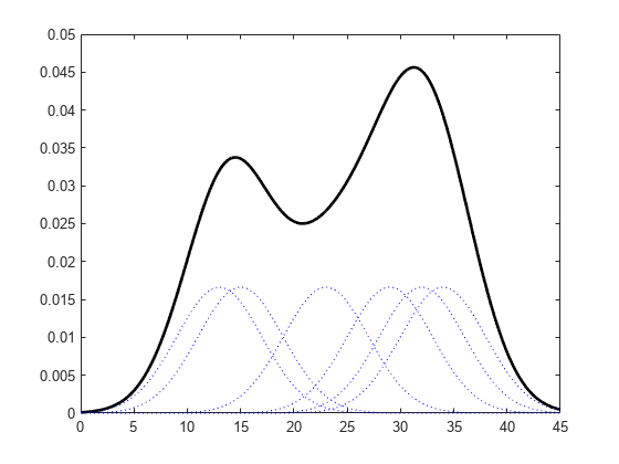
Alternatively, the kernel distribution builds the pdf by creating an individual probability density curve for each data value, then summing the smooth curves. This approach creates one smooth, continuous probability density function for the data set.

figure
pdSix = fitdist(SixMPG,'Kernel','Width',4);
x = 0:.1:45;
ySix = pdf(pdSix,x);
plot(x,ySix,'k-','LineWidth',2)

% Plot each individual pdf and scale its appearance on the plot
hold on
for i=1:6
    pd = makedist('Normal','mu',SixMPG(i),'sigma',4);
    y = pdf(pd,x);
    y = y/6;
    plot(x,y,'b:')
end
hold off

The smaller dashed curves are the probability distributions for each value in the sample data, scaled to fit the plot. The larger solid curve is the overall kernel distribution of the SixMPG data. The kernel smoothing function refers to the shape of those smaller component curves, which have a normal distribution in this example.

You can choose one of several options for the kernel smoothing function. This plot shows the shapes of the available smoothing functions.

% Set plot specifications
hname = {'normal' 'epanechnikov' 'box' 'triangle'};
colors = {'r' 'b' 'g' 'm'};
lines = {'-','-.','--',':'};

% Generate a sample of each kernel smoothing function and plot
data = [0];
figure
for j=1:4
    pd = fitdist(data,'kernel','Kernel',hname{j});
    x = -3:.1:3;
    y = pdf(pd,x);
    plot(x,y,'Color',colors{j},'LineStyle',lines{j})
    hold on
end
legend(hname)
hold off

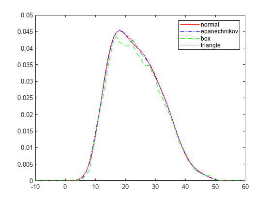
To understand the effect of different kernel smoothing functions on the shape of the resulting pdf estimate, compare plots of the mileage data (MPG) from carbig.mat using each available kernel function.

load carbig
% Set plot specifications
hname = {'normal' 'epanechnikov' 'box' 'triangle'};
colors = {'r' 'b' 'g' 'm'};
lines = {'-','-.','--',':'};

% Generate kernel distribution objects and plot
figure
for j=1:4
    pd = fitdist(MPG,'kernel','Kernel',hname{j});
    x = -10:1:60;
    y = pdf(pd,x);
    plot(x,y,'Color',colors{j},'LineStyle',lines{j})
    hold on
end
legend(hname)
hold off

Each density curve uses the same input data, but applies a different kernel smoothing function to generate the pdf. The density estimates are roughly comparable, but the shape of each curve varies slightly. For example, the box kernel produces a density curve that is less smooth than the others.

Bandwidth

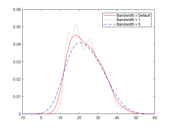
The choice of bandwidth value controls the smoothness of the resulting probability density curve. This plot shows the density estimate for the MPG data, using a normal kernel smoothing function with three different bandwidths.

% Create kernel distribution objects
load carbig
pd1 = fitdist(MPG,'kernel');
pd2 = fitdist(MPG,'kernel','Width',1);
pd3 = fitdist(MPG,'kernel','Width',5);

% Compute each pdf
x = -10:1:60;
y1 = pdf(pd1,x);
y2 = pdf(pd2,x);
y3 = pdf(pd3,x);

% Plot each pdf
plot(x,y1,'Color','r','LineStyle','-')
hold on
plot(x,y2,'Color','k','LineStyle',':')
plot(x,y3,'Color','b','LineStyle','--')
legend({'Bandwidth = Default','Bandwidth = 1','Bandwidth = 5'})
hold off

The default bandwidth, which is theoretically optimal for estimating densities for the normal distribution [1], produces a reasonably smooth curve. Specifying a smaller bandwidth produces a very rough curve, but reveals that there might be two major peaks in the data. Specifying a larger bandwidth produces a curve nearly identical to the kernel function, and is so smooth that it obscures potentially important features of the data.