主要内容

Polynomial Fitting Tool

R2026b

Interactive polynomial fitting

Description

The Polynomial Fitting tool fits a polynomial to two-dimensional data and displays an interactive plot of the result.

You can use the tool to explore the effects of changing the parameters of the fit and to export fit results to the workspace. The tool displays a plot of a polynomial p(x) of degree n that is a best fit (in a least-squares sense) for the data in y. The polynomial p contains n+1 terms, where

p(x)=p1xn+p2xn−1+...+pnx+pn+1.

Required Products

  • MATLAB®

  • Statistics and Machine Learning Toolbox™
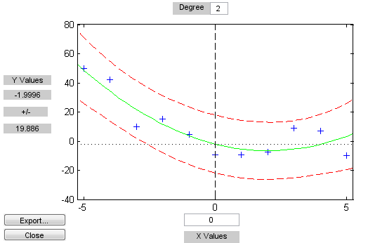
Polynomial Fitting tool

Open the Polynomial Fitting Tool

  • MATLAB command prompt: Enter polytool.

Examples

expand all

This example shows how to start an interactive fitting session with polytool.

Generate data from a quadratic curve with added noise.

rng(0,"twister") % for reproducibility
x = -5:5;
y = x.^2 - 5*x - 3 + 5*randn(size(x));

Fit a quadratic (2nd degree) model with 0.90 confidence intervals.

n = 2;
alpha = 0.1;
polytool(x,y,n,alpha)

Plot of y versus x showing the data points, the fitted model, and its confidence intervals

Parameters

expand all

Specify the polynomial degree as a positive integer.

Change the X value of the crosshair by entering a new value in the field below the plot, or by dragging the vertical line in the plot. The tool updates the corresponding Y value of the fit below the Y axis label.

Use the Bounds menu in the tool window to select the type of confidence bounds: simultaneous or nonsimultaneous, and curve or observation.

  • Simultaneous or Nonsimultaneous

    • Simultaneous (default) — Use Scheffé's method to compute the confidence bounds for the curve of the response values. The range between the upper and lower confidence bounds contains the curve consisting of true response values with 95% confidence.

    • Nonsimultaneous — Compute confidence bounds for the response value at each observation. The confidence interval for a response value at a specific predictor value contains the true response value with 95% confidence.

    With simultaneous bounds, the entire curve of true response values is within the bounds at high confidence. By contrast, nonsimultaneous bounds require only the response value at a single predictor value to be within the bounds at high confidence. Therefore, simultaneous bounds are wider than nonsimultaneous bounds. For more information, see polyconf.

  • Curve or Observation

    • Curve (default) — Plot confidence bounds for the fitted polynomial at the query points x.

    • Observation — Plot confidence bounds for new observations at the values in x.

    In general, Observation (prediction) intervals are wider than Curve (confidence) intervals, due to the additional uncertainty of predicting a new response value (the curve plus random errors). Likewise, simultaneous intervals are wider than nonsimultaneous intervals, due to the additional uncertainty of bounding values for all predictor values of x.

  • Select None if you do not want to display confidence bounds.

Use the Method menu in the tool window to select the fitting method. The Least Squares method uses ordinary least squares fitting, and the Robust method uses robust fitting with the "bisquare" weight function and the default tuning constant. For more information, see robustfit.

Programmatic Use

polytool(x,y) fits a line to the vectors x and y and displays an interactive plot of the result. You can use the interface to explore the effects of changing the parameters of the fit, and to export the fit results to the workspace.

polytool(x,y,n) initially fits a polynomial of degree n. The default is 1, which produces a linear fit.

polytool(x,y,n,alpha) initially plots 100(1–alpha)% confidence intervals on the predicted values. The default value of alpha is 0.05, which results in 95% confidence intervals.

polytool(x,y,n,alpha,xname,yname) labels the x and y values on the plot using xname and yname, respectively. Specify n and alpha as [] to use their default values.

h = polytool(___) outputs a vector of handles h to the line objects in the plot, using any of the input argument combinations in the previous syntaxes.

Tips

  • Click the Export button to export the fitted parameters, confidence intervals, and fit residuals to the workspace. Adjust the variable names and clear any check boxes in the Export to Workspace dialog box, if necessary.

Version History

Introduced before R2006a