incrementalLearner

Convert linear regression model to incremental learner

Syntax

IncrementalMdl = incrementalLearner(Mdl)

IncrementalMdl = incrementalLearner(Mdl,Name,Value)

Description

IncrementalMdl = incrementalLearner(Mdl) returns a linear regression model for incremental learning, IncrementalMdl, using the hyperparameters and coefficients of the traditionally trained linear regression model Mdl. Because its property values reflect the knowledge gained from Mdl, IncrementalMdl can predict labels given new observations, and it is warm, meaning that its predictive performance is tracked.

example

IncrementalMdl = incrementalLearner(Mdl,Name,Value) uses additional options specified by one or more name-value arguments. Some options require you to train IncrementalMdl before its predictive performance is tracked. For example, 'MetricsWarmupPeriod',50,'MetricsWindowSize',100 specifies a preliminary incremental training period of 50 observations before performance metrics are tracked, and specifies processing 100 observations before updating the window performance metrics.

example

Examples

collapse all

Convert Traditionally Trained Model to Incremental Learner

Open Live Script

Train a linear regression model by using fitrlinear, and then convert it to an incremental learner.

Load and Preprocess Data

Load the 2015 NYC housing data set. For more details on the data, see NYC Open Data.

load NYCHousing2015

Extract the response variable SALEPRICE from the table. For numerical stability, scale SALEPRICE by 1e6.

Y = NYCHousing2015.SALEPRICE/1e6;
NYCHousing2015.SALEPRICE = [];

Create dummy variable matrices from the categorical predictors.

catvars = ["BOROUGH" "BUILDINGCLASSCATEGORY" "NEIGHBORHOOD"];
dumvarstbl = varfun(@(x)dummyvar(categorical(x)),NYCHousing2015,...
    'InputVariables',catvars);
dumvarmat = table2array(dumvarstbl);
NYCHousing2015(:,catvars) = [];

Treat all other numeric variables in the table as linear predictors of sales price. Concatenate the matrix of dummy variables to the rest of the predictor data.

idxnum = varfun(@isnumeric,NYCHousing2015,'OutputFormat','uniform');
X = [dumvarmat NYCHousing2015{:,idxnum}];

Train Linear Regression Model

Fit a linear regression model to the entire data set.

TTMdl = fitrlinear(X,Y)

TTMdl = 
  RegressionLinear
         ResponseName: 'Y'
    ResponseTransform: 'none'
                 Beta: [312×1 double]
                 Bias: 0.0956
               Lambda: 1.0935e-05
              Learner: 'svm'


  Properties, Methods

TTMdl is a RegressionLinear model object representing a traditionally trained linear regression model.

Convert Trained Model

Convert the traditionally trained linear regression model to a linear regression model for incremental learning.

IncrementalMdl = incrementalLearner(TTMdl)

IncrementalMdl = 
  incrementalRegressionLinear

               IsWarm: 1
              Metrics: [1×2 table]
    ResponseTransform: 'none'
                 Beta: [312×1 double]
                 Bias: 0.0956
              Learner: 'svm'


  Properties, Methods

IncrementalMdl is an incrementalRegressionLinear model object prepared for incremental learning using SVM.

The incrementalLearner function Initializes the incremental learner by passing learned coefficients to it, along with other information TTMdl extracted from the training data.
IncrementalMdl is warm (IsWarm is 1), which means that incremental learning functions can start tracking performance metrics.
incrementalRegressionLinear trains the model using the adaptive scale-invariant solver, whereas fitrlinear trained TTMdl using the dual SGD solver.

Predict Responses

An incremental learner created from converting a traditionally trained model can generate predictions without further processing.

Predict sales prices for all observations using both models.

ttyfit = predict(TTMdl,X);
ilyfit = predict(IncrementalMdl,X);
compareyfit = norm(ttyfit - ilyfit)

compareyfit = 
0

The difference between the fitted values generated by the models is 0.

Specify SGD Solver

Open Live Script

The default solver is the adaptive scale-invariant solver. If you specify this solver, you do not need to tune any parameters for training. However, if you specify either the standard SGD or ASGD solver instead, you can also specify an estimation period, during which the incremental fitting functions tune the learning rate.

Load and shuffle the 2015 NYC housing data set. For more details on the data, see NYC Open Data.

load NYCHousing2015

rng(1) % For reproducibility
n = size(NYCHousing2015,1);
shuffidx = randsample(n,n);
NYCHousing2015 = NYCHousing2015(shuffidx,:);

Extract the response variable SALEPRICE from the table. For numerical stability, scale SALEPRICE by 1e6.

Y = NYCHousing2015.SALEPRICE/1e6;
NYCHousing2015.SALEPRICE = [];

Create dummy variable matrices from the categorical predictors.

catvars = ["BOROUGH" "BUILDINGCLASSCATEGORY" "NEIGHBORHOOD"];
dumvarstbl = varfun(@(x)dummyvar(categorical(x)),NYCHousing2015,...
    'InputVariables',catvars);
dumvarmat = table2array(dumvarstbl);
NYCHousing2015(:,catvars) = [];

Treat all other numeric variables in the table as linear predictors of sales price. Concatenate the matrix of dummy variables to the rest of the predictor data.

idxnum = varfun(@isnumeric,NYCHousing2015,'OutputFormat','uniform');
X = [dumvarmat NYCHousing2015{:,idxnum}];

Randomly partition the data into 5% and 95% sets: the first set for training a model traditionally, and the second set for incremental learning.

cvp = cvpartition(n,'Holdout',0.95);
idxtt = training(cvp);
idxil = test(cvp);

% 5% set for traditional training 
Xtt = X(idxtt,:);
Ytt = Y(idxtt);

% 95% set for incremental learning
Xil = X(idxil,:);
Yil = Y(idxil);

Fit a linear regression model to 5% of the data.

TTMdl = fitrlinear(Xtt,Ytt);

Convert the traditionally trained linear regression model to a linear regression model for incremental learning. Specify the standard SGD solver and an estimation period of 2e4 observations (the default is 1000 when a learning rate is required).

IncrementalMdl = incrementalLearner(TTMdl,'Solver','sgd','EstimationPeriod',2e4);

IncrementalMdl is an incrementalRegressionLinear model object.

Fit the incremental model to the rest of the data by using the fit function. At each iteration:

Simulate a data stream by processing 10 observations at a time.
Overwrite the previous incremental model with a new one fitted to the incoming observations.
Store the initial learning rate and $β_{1}$ to see how the coefficients and rate evolve during training.

% Preallocation
nil = numel(Yil);
numObsPerChunk = 10;
nchunk = floor(nil/numObsPerChunk);
learnrate = [IncrementalMdl.LearnRate; zeros(nchunk,1)];
beta1 = [IncrementalMdl.Beta(1); zeros(nchunk,1)];    

% Incremental fitting
for j = 1:nchunk
    ibegin = min(nil,numObsPerChunk*(j-1) + 1);
    iend   = min(nil,numObsPerChunk*j);
    idx = ibegin:iend;
    IncrementalMdl = fit(IncrementalMdl,Xil(idx,:),Yil(idx));
    beta1(j + 1) = IncrementalMdl.Beta(1);
    learnrate(j + 1) = IncrementalMdl.LearnRate;
end

IncrementalMdl is an incrementalRegressionLinear model object trained on all the data in the stream.

To see how the initial learning rate and $β_{1}$ evolve during training, plot them on separate tiles.

t = tiledlayout(2,1);
nexttile
plot(beta1)
hold on
ylabel('\beta_1')
xline(IncrementalMdl.EstimationPeriod/numObsPerChunk,'r-.')
nexttile
plot(learnrate)
ylabel('Initial Learning Rate')
xline(IncrementalMdl.EstimationPeriod/numObsPerChunk,'r-.')
xlabel(t,'Iteration')

$Figure contains 2 axes objects. Axes object 1 with ylabel \beta_1 contains 2 objects of type line, constantline. Axes object 2 with ylabel Initial Learning Rate contains 2 objects of type line, constantline.$

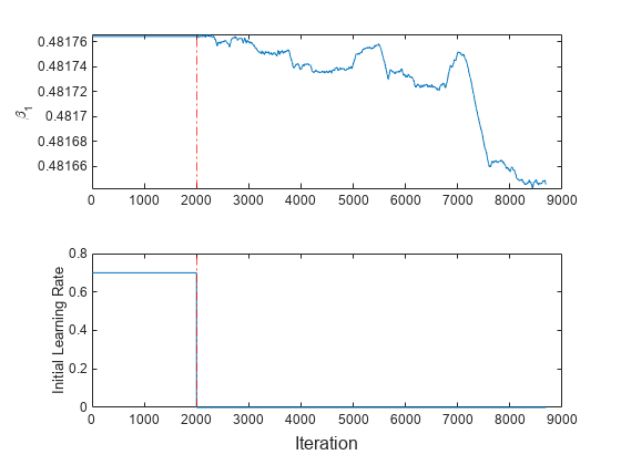
The initial learning rate jumps from 0.7 to its autotuned value after the estimation period. During training, the software uses a learning rate that gradually decays from the initial value specified in the LearnRateSchedule property of IncrementalMdl.

Because fit does not fit the model to the streaming data during the estimation period, $β_{1}$ is constant for the first 2000 iterations (20,000 observations). Then, $β_{1}$ changes slightly as fit fits the model to each new chunk of 10 observations.

Configure Performance Metric Options

Open Live Script

Use a trained linear regression model to initialize an incremental learner. Prepare the incremental learner by specifying a metrics warm-up period, during which the updateMetricsAndFit function only fits the model. Specify a metrics window size of 500 observations.

Load the robot arm data set.

load robotarm

For details on the data set, enter Description at the command line.

Randomly partition the data into 5% and 95% sets: the first set for training a model traditionally, and the second set for incremental learning.

n = numel(ytrain);

rng(1) % For reproducibility
cvp = cvpartition(n,'Holdout',0.95);
idxtt = training(cvp);
idxil = test(cvp);

% 5% set for traditional training
Xtt = Xtrain(idxtt,:);
Ytt = ytrain(idxtt);

% 95% set for incremental learning
Xil = Xtrain(idxil,:);
Yil = ytrain(idxil);

Fit a linear regression model to the first set.

TTMdl = fitrlinear(Xtt,Ytt);

Convert the traditionally trained linear regression model to a linear regression model for incremental learning. Specify the following:

A performance metrics warm-up period of 2000 observations.
A metrics window size of 500 observations.
Use of epsilon insensitive loss, MSE, and mean absolute error (MAE) to measure the performance of the model. The software supports epsilon insensitive loss and MSE. Create an anonymous function that measures the absolute error of each new observation. Create a structure array containing the name MeanAbsoluteError and its corresponding function.

maefcn = @(z,zfit)abs(z - zfit);
maemetric = struct("MeanAbsoluteError",maefcn);
IncrementalMdl = incrementalLearner(TTMdl,'MetricsWarmupPeriod',2000,'MetricsWindowSize',500,...
    'Metrics',{'epsiloninsensitive' 'mse' maemetric});

Fit the incremental model to the rest of the data by using the updateMetricsAndFit function. At each iteration:

Simulate a data stream by processing 50 observations at a time.
Overwrite the previous incremental model with a new one fitted to the incoming observations.
Store $β_{10}$ , the cumulative metrics, and the window metrics to see how they evolve during incremental learning.

% Preallocation
nil = numel(Yil);
numObsPerChunk = 50;
nchunk = floor(nil/numObsPerChunk);
ei = array2table(zeros(nchunk,2),'VariableNames',["Cumulative" "Window"]);
mse = array2table(zeros(nchunk,2),'VariableNames',["Cumulative" "Window"]);
mae = array2table(zeros(nchunk,2),'VariableNames',["Cumulative" "Window"]);
beta1 = zeros(nchunk+1,1);    
beta1(1) = IncrementalMdl.Beta(10);

% Incremental fitting
for j = 1:nchunk
    ibegin = min(nil,numObsPerChunk*(j-1) + 1);
    iend   = min(nil,numObsPerChunk*j);
    idx = ibegin:iend;    
    IncrementalMdl = updateMetricsAndFit(IncrementalMdl,Xil(idx,:),Yil(idx));
    ei{j,:} = IncrementalMdl.Metrics{"EpsilonInsensitiveLoss",:};
    mse{j,:} = IncrementalMdl.Metrics{"MeanSquaredError",:};
    mae{j,:} = IncrementalMdl.Metrics{"MeanAbsoluteError",:};
    beta1(j + 1) = IncrementalMdl.Beta(10);
end

IncrementalMdl is an incrementalRegressionLinear model object trained on all the data in the stream. During incremental learning and after the model is warmed up, updateMetricsAndFit checks the performance of the model on the incoming observations, and then fits the model to those observations.

To see how the performance metrics and $β_{10}$ evolve during training, plot them on separate tiles.

tiledlayout(2,2)
nexttile
plot(beta1)
ylabel('\beta_{10}')
xlim([0 nchunk])
xline(IncrementalMdl.MetricsWarmupPeriod/numObsPerChunk,'r-.')
xlabel('Iteration')
nexttile
h = plot(ei.Variables);
xlim([0 nchunk])
ylabel('Epsilon Insensitive Loss')
xline(IncrementalMdl.MetricsWarmupPeriod/numObsPerChunk,'r-.')
legend(h,ei.Properties.VariableNames)
xlabel('Iteration')
nexttile
h = plot(mse.Variables);
xlim([0 nchunk]);
ylabel('MSE')
xline(IncrementalMdl.MetricsWarmupPeriod/numObsPerChunk,'r-.')
legend(h,mse.Properties.VariableNames)
xlabel('Iteration')
nexttile
h = plot(mae.Variables);
xlim([0 nchunk]);
ylabel('MAE')
xline(IncrementalMdl.MetricsWarmupPeriod/numObsPerChunk,'r-.')
legend(h,mae.Properties.VariableNames)
xlabel('Iteration')

$Figure contains 4 axes objects. Axes object 1 with xlabel Iteration, ylabel \beta_{10} contains 2 objects of type line, constantline. Axes object 2 with xlabel Iteration, ylabel Epsilon Insensitive Loss contains 3 objects of type line, constantline. These objects represent Cumulative, Window. Axes object 3 with xlabel Iteration, ylabel MSE contains 3 objects of type line, constantline. These objects represent Cumulative, Window. Axes object 4 with xlabel Iteration, ylabel MAE contains 3 objects of type line, constantline. These objects represent Cumulative, Window.$

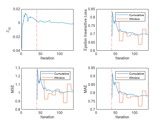
The plot suggests that updateMetricsAndFit does the following:

Fit $β_{10}$ during all incremental learning iterations.
Compute the performance metrics after the metrics warm-up period only.
Compute the cumulative metrics during each iteration.
Compute the window metrics after processing 500 observations.

Input Arguments

collapse all

`Mdl` — Traditionally trained linear regression model
`RegressionLinear` model object

Traditionally trained linear regression model, specified as a RegressionLinear model object returned by fitrlinear.

Note

If Mdl.Lambda is a numeric vector, you must select the model corresponding to one regularization strength in the regularization path by using selectModels.
Incremental learning functions support only numeric input predictor data. If Mdl was trained on categorical data, you must prepare an encoded version of the categorical data to use incremental learning functions. Use dummyvar to convert each categorical variable to a numeric matrix of dummy variables. Then, concatenate all dummy variable matrices and any other numeric predictors, in the same way that the training function encodes categorical data. For more details, see Dummy Variables.

Name-Value Arguments

expand all

Specify optional pairs of arguments as Name1=Value1,...,NameN=ValueN, where Name is the argument name and Value is the corresponding value. Name-value arguments must appear after other arguments, but the order of the pairs does not matter.

Before R2021a, use commas to separate each name and value, and enclose Name in quotes.

Example: 'Solver','scale-invariant','MetricsWindowSize',100 specifies the adaptive scale-invariant solver for objective optimization, and specifies processing 100 observations before updating the window performance metrics.

General Options

expand all

`Solver` — Objective function minimization technique
`'scale-invariant'` | `'sgd'` | `'asgd'`

Objective function minimization technique, specified as the comma-separated pair consisting of 'Solver' and a value in this table.

Value Description Notes

Value	Description	Notes
`'scale-invariant'`	Adaptive scale-invariant solver for incremental learning [1]	This algorithm is parameter free and can adapt to differences in predictor scales. Try this algorithm before using SGD or ASGD. To shuffle an incoming chunk of data before the `fit` function fits the model, set `Shuffle` to `true`.
`'sgd'`	Stochastic gradient descent (SGD) [3][2]	To train effectively with SGD, standardize the data and specify adequate values for hyperparameters using options listed in SGD and ASGD Solver Options. The `fit` function always shuffles an incoming chunk of data before fitting the model.
`'asgd'`	Average stochastic gradient descent (ASGD) [4]	To train effectively with ASGD, standardize the data and specify adequate values for hyperparameters using options listed in SGD and ASGD Solver Options. The `fit` function always shuffles an incoming chunk of data before fitting the model.

'scale-invariant'

Adaptive scale-invariant solver for incremental learning [1]

This algorithm is parameter free and can adapt to differences in predictor scales. Try this algorithm before using SGD or ASGD.
To shuffle an incoming chunk of data before the fit function fits the model, set Shuffle to true.

'sgd'

Stochastic gradient descent (SGD) [3][2]

To train effectively with SGD, standardize the data and specify adequate values for hyperparameters using options listed in SGD and ASGD Solver Options.
The fit function always shuffles an incoming chunk of data before fitting the model.

'asgd'

Average stochastic gradient descent (ASGD) [4]

To train effectively with ASGD, standardize the data and specify adequate values for hyperparameters using options listed in SGD and ASGD Solver Options.
The fit function always shuffles an incoming chunk of data before fitting the model.

If Mdl.Regularization is 'ridge (L2)' and Mdl.ModelParameters.Solver is 'sgd' or 'asgd', the default Solver value is Mdl.ModelParameters.Solver.
Otherwise, the default Solver value is 'scale-invariant'.

Example: 'Solver','sgd'

Data Types: char | string

`EstimationPeriod` — Number of observations processed to estimate hyperparameters
nonnegative integer

Number of observations processed by the incremental model to estimate hyperparameters before training or tracking performance metrics, specified as the comma-separated pair consisting of 'EstimationPeriod' and a nonnegative integer.

Note

If Mdl is prepared for incremental learning (all hyperparameters required for training are specified), incrementalLearner forces EstimationPeriod to 0.
If Mdl is not prepared for incremental learning, incrementalLearner sets EstimationPeriod to 1000.

For more details, see Estimation Period.

Example: 'EstimationPeriod',100

Data Types: single | double

SGD and ASGD Solver Options

expand all

`BatchSize` — Mini-batch size
positive integer

Mini-batch size, specified as the comma-separated pair consisting of 'BatchSize' and a positive integer. At each learning cycle during training, incrementalLearner uses BatchSize observations to compute the subgradient.

The number of observations for the last mini-batch (last learning cycle in each function call of fit or updateMetricsAndFit) can be smaller than BatchSize. For example, if you supply 25 observations to fit or updateMetricsAndFit, the function uses 10 observations for the first two learning cycles and uses 5 observations for the last learning cycle.

If Mdl.Regularization is 'ridge (L2)' and Mdl.ModelParameters.Solver is 'sgd' or 'asgd', you cannot set BatchSize. Instead, incrementalLearner sets BatchSize to Mdl.ModelParameters.BatchSize.
Otherwise, BatchSize is 10.

Example: 'BatchSize',1

Data Types: single | double

`Lambda` — Ridge (L2) regularization term strength
nonnegative scalar

Ridge (L2) regularization term strength, specified as the comma-separated pair consisting of 'Lambda' and a nonnegative scalar.

If Mdl.Regularization is 'ridge (L2)' and Mdl.ModelParameters.Solver is 'sgd' or 'asgd', you cannot set Lambda. Instead, incrementalLearner sets Lambda to Mdl.Lambda.
Otherwise, Lambda is 1e-5.

Note

incrementalLearner does not support lasso regularization. If Mdl.Regularization is 'lasso (L1)', incrementalLearner uses ridge regularization instead, and sets the Solver name-value pair argument to 'scale-invariant' by default.

Example: 'Lambda',0.01

Data Types: single | double

`LearnRate` — Initial learning rate
`'auto'` | positive scalar

Initial learning rate, specified as the comma-separated pair consisting of 'LearnRate' and 'auto' or a positive scalar.

The learning rate controls the optimization step size by scaling the objective subgradient. LearnRate specifies an initial value for the learning rate, and LearnRateSchedule determines the learning rate for subsequent learning cycles.

When you specify 'auto':

The initial learning rate is 0.7.
If EstimationPeriod > 0, fit and updateMetricsAndFit change the rate to 1/sqrt(1+max(sum(X.^2,obsDim))) at the end of EstimationPeriod. When the observations are the columns of the predictor data X collected during the estimation period, the obsDim value is 1; otherwise, the value is 2.

By default:

If Mdl.Regularization is 'ridge (L2)' and Mdl.ModelParameters.Solver is 'sgd' or 'asgd', you cannot set LearnRate. Instead, incrementalLearner sets LearnRate to Mdl.ModelParameters.LearnRate.
Otherwise, LearnRate is 'auto'.

Example: 'LearnRate',0.001

Data Types: single | double | char | string

`LearnRateSchedule` — Learning rate schedule
`'decaying'` (default) | `'constant'`

Learning rate schedule, specified as the comma-separated pair consisting of 'LearnRateSchedule' and a value in this table, where LearnRate specifies the initial learning rate ɣ₀.

Value Description

'constant' The learning rate is ɣ₀ for all learning cycles.

Value	Description
`'constant'`	The learning rate is ɣ₀ for all learning cycles.
`'decaying'`	The learning rate at learning cycle t is $γ_{t} = \frac{γ_{0}}{{(1 + λ γ_{0} t)}^{c}} .$ λ is the value of `Lambda`. If `Solver` is `'sgd'`, c = `1`. If `Solver` is `'asgd'`: c = `2/3` if `Learner` is `'leastsquares'`. c = `3/4` if `Learner` is `'svm'` [4].

'decaying'

The learning rate at learning cycle t is

$γ_{t} = \frac{γ_{0}}{{(1 + λ γ_{0} t)}^{c}} .$

λ is the value of Lambda.
If Solver is 'sgd', c = 1.
If Solver is 'asgd':
- c = 2/3 if Learner is 'leastsquares'.
- c = 3/4 if Learner is 'svm' [4].

If Mdl.Regularization is 'ridge (L2)' and Mdl.ModelParameters.Solver is 'sgd' or 'asgd', you cannot set LearnRateSchedule. Instead, incrementalLearner sets LearnRateSchedule to 'decaying'.

Example: 'LearnRateSchedule','constant'

Data Types: char | string

Adaptive Scale-Invariant Solver Options

expand all

`Shuffle` — Flag for shuffling observations in batch
`true` (default) | `false`

Flag for shuffling the observations in the batch at each iteration, specified as the comma-separated pair consisting of 'Shuffle' and a value in this table.

Value	Description
`true`	The software shuffles an incoming chunk of data before the `fit` function fits the model. This action reduces bias induced by the sampling scheme.
`false`	The software processes the data in the order received.

Example: 'Shuffle',false

Data Types: logical

Performance Metrics Options

expand all

`Metrics` — Model performance metrics to track during incremental learning
`"epsiloninsensitive"` | `"mse"` | string vector | function handle | cell vector | structure array

Model performance metrics to track during incremental learning with updateMetrics and updateMetricsAndFit, specified as the comma-separated pair consisting of 'Metrics' and a built-in loss function name, string vector of names, function handle (@metricName), structure array of function handles, or cell vector of names, function handles, or structure arrays.

The following table lists the built-in loss function names and which learners, specified in Mdl.Learner, support them. You can specify more than one loss function by using a string vector.

Name	Description	Learner Supporting Metric
`"epsiloninsensitive"`	Epsilon insensitive loss	`'svm'`
`"mse"`	Weighted mean squared error	`'svm'` and `'leastsquares'`

For more details on the built-in loss functions, see loss.

Example: 'Metrics',["epsiloninsensitive" "mse"]

To specify a custom function that returns a performance metric, use function handle notation. The function must have this form:

metric = customMetric(Y,YFit)

The output argument metric is an n-by-1 numeric vector, where each element is the loss of the corresponding observation in the data processed by the incremental learning functions during a learning cycle.
You specify the function name (customMetric).
Y is a length n numeric vector of observed responses, where n is the sample size.
YFit is a length n numeric vector of corresponding predicted responses.

To specify multiple custom metrics and assign a custom name to each, use a structure array. To specify a combination of built-in and custom metrics, use a cell vector.

Example: 'Metrics',struct('Metric1',@customMetric1,'Metric2',@customMetric2)

Example: 'Metrics',{@customMetric1 @customMetric2 'mse' struct('Metric3',@customMetric3)}

updateMetrics and updateMetricsAndFit store specified metrics in a table in the property IncrementalMdl.Metrics. The data type of Metrics determines the row names of the table.

`'Metrics'` Value Data Type	Description of `Metrics` Property Row Name	Example
String or character vector	Name of corresponding built-in metric	Row name for `"epsiloninsensitive"` is `"EpsilonInsensitiveLoss"`
Structure array	Field name	Row name for `struct('Metric1',@customMetric1)` is `"Metric1"`
Function handle to function stored in a program file	Name of function	Row name for `@customMetric` is `"customMetric"`
Anonymous function	`CustomMetric_j`, where `j` is metric `j` in `Metrics`	Row name for `@(Y,YFit)customMetric(Y,YFit)...` is `CustomMetric_1`

By default:

Metrics is "epsiloninsensitive" if Mdl.Learner is 'svm'.
Metrics is "mse" if Mdl.Learner is 'leastsquares'.

For more details on performance metrics options, see Performance Metrics.

Data Types: char | string | struct | cell | function_handle

`MetricsWarmupPeriod` — Number of observations fit before tracking performance metrics
`0` (default) | nonnegative integer

Number of observations the incremental model must be fit to before it tracks performance metrics in its Metrics property, specified as a nonnegative integer. The incremental model is warm after incremental fitting functions fit (EstimationPeriod + MetricsWarmupPeriod) observations to the incremental model.

For more details on performance metrics options, see Performance Metrics.

Example: 'MetricsWarmupPeriod',50

Data Types: single | double

`MetricsWindowSize` — Number of observations to use to compute window performance metrics
`200` (default) | positive integer

Number of observations to use to compute window performance metrics, specified as a positive integer.

For more details on performance metrics options, see Performance Metrics.

Example: 'MetricsWindowSize',100

Data Types: single | double

Output Arguments

collapse all

`IncrementalMdl` — Linear regression model for incremental learning
`incrementalRegressionLinear` model object

Linear regression model for incremental learning, returned as an incrementalRegressionLinear model object. IncrementalMdl is also configured to generate predictions given new data (see predict).

To initialize IncrementalMdl for incremental learning, incrementalLearner passes the values of the Mdl properties in this table to corresponding properties of IncrementalMdl.

Property	Description
`Beta`	Linear model coefficients, a numeric vector
`Bias`	Model intercept, a numeric scalar
`Epsilon`	Half the width of the epsilon insensitive band, a nonnegative scalar
`Learner`	Linear regression model type, a character vector
`ModelParameters.FitBias`	Linear model intercept inclusion flag
`NumPredictors`	Number of predictors, a positive integer
`ResponseTransform`	Response transformation function, a function name or function handle

If Mdl.Regularization is 'ridge (L2)' and Mdl.ModelParameters.Solver is 'sgd' or 'asgd', incrementalLearner also passes the values of Mdl properties in this table.

Property	Description
`Lambda`	Ridge (L2) regularization term strength, a nonnegative scalar
`ModelParameters.LearnRate`	Learning rate, a positive scalar
`ModelParameters.BatchSize`	Mini-batch size, a positive integer
`ModelParameters.Solver`	Objective function minimization technique, a character vector

More About

collapse all

Incremental Learning

Incremental learning, or online learning, is a branch of machine learning concerned with processing incoming data from a data stream, possibly given little to no knowledge of the distribution of the predictor variables, aspects of the prediction or objective function (including tuning parameter values), or whether the observations are labeled. Incremental learning differs from traditional machine learning, where enough labeled data is available to fit to a model, perform cross-validation to tune hyperparameters, and infer the predictor distribution.

Given incoming observations, an incremental learning model processes data in any of the following ways, but usually in this order:

Predict labels.
Measure the predictive performance.
Check for structural breaks or drift in the model.
Fit the model to the incoming observations.

For more details, see Incremental Learning Overview.

Adaptive Scale-Invariant Solver for Incremental Learning

The adaptive scale-invariant solver for incremental learning, introduced in [1], is a gradient-descent-based objective solver for training linear predictive models. The solver is hyperparameter free, insensitive to differences in predictor variable scales, and does not require prior knowledge of the distribution of the predictor variables. These characteristics make it well suited to incremental learning.

The standard SGD and ASGD solvers are sensitive to differing scales among the predictor variables, resulting in models that can perform poorly. To achieve better accuracy using SGD and ASGD, you can standardize the predictor data, and tune the regularization and learning rate parameters. For traditional machine learning, enough data is available to enable hyperparameter tuning by cross-validation and predictor standardization. However, for incremental learning, enough data might not be available (for example, observations might be available only one at a time) and the distribution of the predictors might be unknown. These characteristics make parameter tuning and predictor standardization difficult or impossible to do during incremental learning.

The incremental fitting functions for regression fit and updateMetricsAndFit use the more conservative ScInOL1 version of the algorithm.

Algorithms

collapse all

Estimation Period

During the estimation period, the incremental fitting functions fit and updateMetricsAndFit use the first incoming EstimationPeriod observations to estimate (tune) hyperparameters required for incremental training. Estimation occurs only when EstimationPeriod is positive. This table describes the hyperparameters and when they are estimated, or tuned.

Hyperparameter Model Property Usage Conditions

Predictor means and standard deviations

Hyperparameter	Model Property	Usage	Conditions
Predictor means and standard deviations	`Mu` and `Sigma`	Standardize predictor data	The hyperparameters are not estimated.
Learning rate	`LearnRate`	Adjust the solver step size	The hyperparameter is estimated when both of these conditions apply: You change the solver of `Mdl` to SGD or ASGD (see `Solver`). You do not specify the `'LearnRate'` name-value argument as a positive scalar.

Mu and Sigma

Standardize predictor data

The hyperparameters are not estimated.

Learning rate

LearnRate

Adjust the solver step size

The hyperparameter is estimated when both of these conditions apply:

You change the solver of Mdl to SGD or ASGD (see Solver).
You do not specify the 'LearnRate' name-value argument as a positive scalar.

During the estimation period, fit does not fit the model, and updateMetricsAndFit does not fit the model or update the performance metrics. At the end of the estimation period, the functions update the properties that store the hyperparameters.

Standardize Data

If incremental learning functions are configured to standardize predictor variables, they do so using the means and standard deviations stored in the Mu and Sigma properties of the incremental learning model IncrementalMdl.

If you standardize the predictor data when you train the input model Mdl by using fitrlinear, the following conditions apply:
- incrementalLearner passes the means in Mdl.Mu and standard deviations in Mdl.Sigma to the corresponding incremental learning model properties.
- Incremental learning functions always standardize the predictor data.
When incremental fitting functions estimate predictor means and standard deviations, the functions compute weighted means and weighted standard deviations using the estimation period observations. Specifically, the functions standardize predictor j (x_j) using

$x_{j}^{*} = \frac{x_{j} - μ_{j}^{*}}{σ_{j}^{*}} .$
where
- x_j is predictor j, and x_jk is observation k of predictor j in the estimation period.
- $μ_{j}^{*} = \frac{1}{\sum_{k} w_{k}} \sum_{k} w_{k} x_{j k} .$
- ${(σ_{j}^{*})}^{2} = \frac{1}{\sum_{k} w_{k}} \sum_{k} w_{k} {(x_{j k} - μ_{j}^{*})}^{2} .$
- w_j is observation weight j.

Performance Metrics

The updateMetrics and updateMetricsAndFit functions are incremental learning functions that track model performance metrics ('Metrics') from new data when the incremental model is warm (IsWarm property). An incremental model becomes warm after fit or updateMetricsAndFit fit the incremental model to 'MetricsWarmupPeriod' observations, which is the metrics warm-up period.
If 'EstimationPeriod' > 0, the functions estimate hyperparameters before fitting the model to data. Therefore, the functions must process an additional EstimationPeriod observations before the model starts the metrics warm-up period.
The Metrics property of the incremental model stores two forms of each performance metric as variables (columns) of a table, Cumulative and Window, with individual metrics in rows. When the incremental model is warm, updateMetrics and updateMetricsAndFit update the metrics at the following frequencies:
- Cumulative — The functions compute cumulative metrics since the start of model performance tracking. The functions update metrics every time you call the functions and base the calculation on the entire supplied data set.
- Window — The functions compute metrics based on all observations within a window determined by the 'MetricsWindowSize' name-value pair argument. 'MetricsWindowSize' also determines the frequency at which the software updates Window metrics. For example, if MetricsWindowSize is 20, the functions compute metrics based on the last 20 observations in the supplied data (X((end – 20 + 1):end,:) and Y((end – 20 + 1):end)).
  Incremental functions that track performance metrics within a window use the following process:
  1. Store a buffer of length MetricsWindowSize for each specified metric, and store a buffer of observation weights.
  2. Populate elements of the metrics buffer with the model performance based on batches of incoming observations, and store corresponding observation weights in the weights buffer.
  3. When the buffer is filled, overwrite IncrementalMdl.Metrics.Window with the weighted average performance in the metrics window. If the buffer is overfilled when the function processes a batch of observations, the latest incoming MetricsWindowSize observations enter the buffer, and the earliest observations are removed from the buffer. For example, suppose MetricsWindowSize is 20, the metrics buffer has 10 values from a previously processed batch, and 15 values are incoming. To compose the length 20 window, the functions use the measurements from the 15 incoming observations and the latest 5 measurements from the previous batch.

The software omits an observation with a NaN prediction when computing the Cumulative and Window performance metric values.

References

[1] Kempka, Michał, Wojciech Kotłowski, and Manfred K. Warmuth. "Adaptive Scale-Invariant Online Algorithms for Learning Linear Models." Preprint, submitted February 10, 2019. https://arxiv.org/abs/1902.07528.

[2] Langford, J., L. Li, and T. Zhang. “Sparse Online Learning Via Truncated Gradient.” J. Mach. Learn. Res., Vol. 10, 2009, pp. 777–801.

[3] Shalev-Shwartz, S., Y. Singer, and N. Srebro. “Pegasos: Primal Estimated Sub-Gradient Solver for SVM.” Proceedings of the 24th International Conference on Machine Learning, ICML ’07, 2007, pp. 807–814.

[4] Xu, Wei. “Towards Optimal One Pass Large Scale Learning with Averaged Stochastic Gradient Descent.” CoRR, abs/1107.2490, 2011.

Version History

Introduced in R2020b

incrementalLearner

Syntax

Description

Examples

Convert Traditionally Trained Model to Incremental Learner

Specify SGD Solver

Configure Performance Metric Options

Input Arguments

`Mdl` — Traditionally trained linear regression model
`RegressionLinear` model object

Name-Value Arguments

General Options

`Solver` — Objective function minimization technique
`'scale-invariant'` | `'sgd'` | `'asgd'`

`EstimationPeriod` — Number of observations processed to estimate hyperparameters
nonnegative integer

SGD and ASGD Solver Options

`BatchSize` — Mini-batch size
positive integer

`Lambda` — Ridge (L2) regularization term strength
nonnegative scalar

`LearnRate` — Initial learning rate
`'auto'` | positive scalar

`LearnRateSchedule` — Learning rate schedule
`'decaying'` (default) | `'constant'`

Adaptive Scale-Invariant Solver Options

`Shuffle` — Flag for shuffling observations in batch
`true` (default) | `false`

Performance Metrics Options

`Metrics` — Model performance metrics to track during incremental learning
`"epsiloninsensitive"` | `"mse"` | string vector | function handle | cell vector | structure array

`MetricsWarmupPeriod` — Number of observations fit before tracking performance metrics
`0` (default) | nonnegative integer

`MetricsWindowSize` — Number of observations to use to compute window performance metrics
`200` (default) | positive integer

Output Arguments

`IncrementalMdl` — Linear regression model for incremental learning
`incrementalRegressionLinear` model object

More About

Incremental Learning

Adaptive Scale-Invariant Solver for Incremental Learning

Algorithms

Estimation Period

Standardize Data

Performance Metrics

References

Version History

See Also

Objects

Functions

Topics

incrementalLearner

Syntax

Description

Examples

Convert Traditionally Trained Model to Incremental Learner

Specify SGD Solver

Configure Performance Metric Options

Input Arguments

Mdl — Traditionally trained linear regression model RegressionLinear model object

Name-Value Arguments

General Options

Solver — Objective function minimization technique 'scale-invariant' | 'sgd' | 'asgd'

EstimationPeriod — Number of observations processed to estimate hyperparameters nonnegative integer

SGD and ASGD Solver Options

BatchSize — Mini-batch size positive integer

Lambda — Ridge (L2) regularization term strength nonnegative scalar

LearnRate — Initial learning rate 'auto' | positive scalar

LearnRateSchedule — Learning rate schedule 'decaying' (default) | 'constant'

Adaptive Scale-Invariant Solver Options

Shuffle — Flag for shuffling observations in batch true (default) | false

Performance Metrics Options

Metrics — Model performance metrics to track during incremental learning "epsiloninsensitive" | "mse" | string vector | function handle | cell vector | structure array

MetricsWarmupPeriod — Number of observations fit before tracking performance metrics 0 (default) | nonnegative integer

MetricsWindowSize — Number of observations to use to compute window performance metrics 200 (default) | positive integer

Output Arguments

IncrementalMdl — Linear regression model for incremental learning incrementalRegressionLinear model object

More About

Incremental Learning

Adaptive Scale-Invariant Solver for Incremental Learning

Algorithms

Estimation Period

Standardize Data

Performance Metrics

References

Version History

See Also

Objects

Functions

Topics

`Mdl` — Traditionally trained linear regression model
`RegressionLinear` model object

`Solver` — Objective function minimization technique
`'scale-invariant'` | `'sgd'` | `'asgd'`

`EstimationPeriod` — Number of observations processed to estimate hyperparameters
nonnegative integer

`BatchSize` — Mini-batch size
positive integer

`Lambda` — Ridge (L2) regularization term strength
nonnegative scalar

`LearnRate` — Initial learning rate
`'auto'` | positive scalar

`LearnRateSchedule` — Learning rate schedule
`'decaying'` (default) | `'constant'`

`Shuffle` — Flag for shuffling observations in batch
`true` (default) | `false`

`Metrics` — Model performance metrics to track during incremental learning
`"epsiloninsensitive"` | `"mse"` | string vector | function handle | cell vector | structure array

`MetricsWarmupPeriod` — Number of observations fit before tracking performance metrics
`0` (default) | nonnegative integer

`MetricsWindowSize` — Number of observations to use to compute window performance metrics
`200` (default) | positive integer

`IncrementalMdl` — Linear regression model for incremental learning
`incrementalRegressionLinear` model object