predict

Predict test set response values by using a trained regression neural network model.

Load the patients data set. Create a table from the data set. Each row corresponds to one patient, and each column corresponds to a diagnostic variable. Use the Systolic variable as the response variable, and the rest of the variables as predictors.

load patients
tbl = table(Diastolic,Height,Smoker,Weight,Systolic);

Separate the data into a training set tblTrain and a test set tblTest by using a nonstratified holdout partition. The software reserves approximately 30% of the observations for the test data set and uses the rest of the observations for the training data set.

rng("default") % For reproducibility of the partition
c = cvpartition(size(tbl,1),"Holdout",0.30);
trainingIndices = training(c);
testIndices = test(c);
tblTrain = tbl(trainingIndices,:);
tblTest = tbl(testIndices,:);

Train a regression neural network model using the training set. Specify the Systolic column of tblTrain as the response variable. Specify to standardize the numeric predictors, and set the iteration limit to 50. By default, the neural network model has one fully connected layer with 10 outputs, excluding the final fully connected layer.

Mdl = fitrnet(tblTrain,"Systolic", ...
    "Standardize",true,"IterationLimit",50);

Predict the systolic blood pressure levels for patients in the test set.

predictedY = predict(Mdl,tblTest);

Visualize the results by using a scatter plot with a reference line. Plot the predicted values along the vertical axis and the true response values along the horizontal axis. Points on the reference line indicate correct predictions.

plot(tblTest.Systolic,predictedY,".")
hold on
plot(tblTest.Systolic,tblTest.Systolic)
hold off
xlabel("True Systolic Blood Pressure Levels")
ylabel("Predicted Systolic Blood Pressure Levels")

Because many of the points are far from the reference line, the default neural network model with a fully connected layer of size 10 does not seem to be a great predictor of systolic blood pressure levels.

Perform feature selection by comparing test set losses and predictions. Compare the test set metrics for a regression neural network model trained using all the predictors to the test set metrics for a model trained using only a subset of the predictors.

Load the sample file fisheriris.csv, which contains iris data including sepal length, sepal width, petal length, petal width, and species type. Read the file into a table.

fishertable = readtable('fisheriris.csv');

Separate the data into a training set trainTbl and a test set testTbl by using a nonstratified holdout partition. The software reserves approximately 30% of the observations for the test data set and uses the rest of the observations for the training data set.

rng("default")
c = cvpartition(size(fishertable,1),"Holdout",0.3);
trainTbl = fishertable(training(c),:);
testTbl = fishertable(test(c),:);

Train one regression neural network model using all the predictors in the training set, and train another model using all the predictors except PetalWidth. For both models, specify PetalLength as the response variable, and standardize the predictors.

allMdl = fitrnet(trainTbl,"PetalLength","Standardize",true);
subsetMdl = fitrnet(trainTbl,"PetalLength ~ SepalLength + SepalWidth + Species", ...
    "Standardize",true);

Compare the test set mean squared error (MSE) of the two models. Smaller MSE values indicate better performance.

allMSE = loss(allMdl,testTbl)

allMSE = 0.0834

subsetMSE = loss(subsetMdl,testTbl)

subsetMSE = 0.0884

For each model, compare the test set predicted petal lengths to the true petal lengths. Plot the predicted petal lengths along the vertical axis and the true petal lengths along the horizontal axis. Points on the reference line indicate correct predictions.

tiledlayout(2,1)

% Top axes
ax1 = nexttile;
allPredictedY = predict(allMdl,testTbl);
plot(ax1,testTbl.PetalLength,allPredictedY,".")
hold on
plot(ax1,testTbl.PetalLength,testTbl.PetalLength)
hold off
xlabel(ax1,"True Petal Length")
ylabel(ax1,"Predicted Petal Length")
title(ax1,"All Predictors")

% Bottom axes
ax2 = nexttile;
subsetPredictedY = predict(subsetMdl,testTbl);
plot(ax2,testTbl.PetalLength,subsetPredictedY,".")
hold on
plot(ax2,testTbl.PetalLength,testTbl.PetalLength)
hold off
xlabel(ax2,"True Petal Length")
ylabel(ax2,"Predicted Petal Length")
title(ax2,"Subset of Predictors")

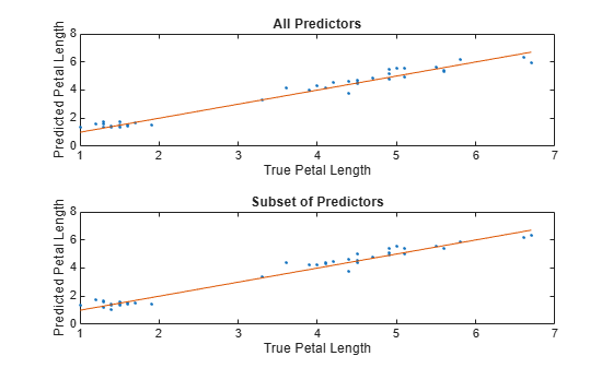
Because both models seems to perform well, with predictions scattered near the reference line, consider using the model trained using all predictors except PetalWidth.

See how the layers of a regression neural network model work together to predict the response value for a single observation.

Load the sample file fisheriris.csv, which contains iris data including sepal length, sepal width, petal length, petal width, and species type. Read the file into a table, and display the first few rows of the table.

fishertable = readtable('fisheriris.csv');
head(fishertable)

    SepalLength    SepalWidth    PetalLength    PetalWidth     Species  
    ___________    __________    ___________    __________    __________

        5.1           3.5            1.4           0.2        {'setosa'}
        4.9             3            1.4           0.2        {'setosa'}
        4.7           3.2            1.3           0.2        {'setosa'}
        4.6           3.1            1.5           0.2        {'setosa'}
          5           3.6            1.4           0.2        {'setosa'}
        5.4           3.9            1.7           0.4        {'setosa'}
        4.6           3.4            1.4           0.3        {'setosa'}
          5           3.4            1.5           0.2        {'setosa'}

Train a regression neural network model using the data set. Specify the PetalLength variable as the response and use the other numeric variables as predictors.

Mdl = fitrnet(fishertable,"PetalLength ~ SepalLength + SepalWidth + PetalWidth");

Select the fifteenth observation from the data set. See how the layers of the neural network take the observation and return a predicted response value newPointResponse.

newPoint = Mdl.X{15,:}

newPoint = 1×3

    5.8000    4.0000    0.2000

firstFCStep = (Mdl.LayerWeights{1})*newPoint' + Mdl.LayerBiases{1};
reluStep = max(firstFCStep,0);

finalFCStep = (Mdl.LayerWeights{end})*reluStep + Mdl.LayerBiases{end};

newPointResponse = finalFCStep

newPointResponse = 1.6716

Check that the prediction matches the one returned by the predict object function.

predictedY = predict(Mdl,newPoint)

predictedY = 1.6716

isequal(newPointResponse,predictedY)

ans = logical
   1

The two results match.