Tune RobustBoost
The RobustBoost algorithm can make good classification predictions even when the training data has noise. However, the default RobustBoost parameters can produce an ensemble that does not predict well. This example shows one way of tuning the parameters for better predictive accuracy.
Generate data with label noise. This example has twenty uniform random numbers per observation, and classifies the observation as 1 if the sum of the first five numbers exceeds 2.5 (so is larger than average), and 0 otherwise:
rng(0,'twister') % for reproducibility
Xtrain = rand(2000,20);
Ytrain = sum(Xtrain(:,1:5),2) > 2.5;
To add noise, randomly switch 10% of the classifications:
idx = randsample(2000,200);
Ytrain(idx) = ~Ytrain(idx);
Create an ensemble with AdaBoostM1 for comparison purposes:
ada = fitcensemble(Xtrain,Ytrain,'Method','AdaBoostM1', ...
    'NumLearningCycles',300,'Learners','Tree','LearnRate',0.1);
Create an ensemble with RobustBoost. Because the data has 10% incorrect classification, perhaps an error goal of 15% is reasonable.
rb1 = fitcensemble(Xtrain,Ytrain,'Method','RobustBoost', ...
    'NumLearningCycles',300,'Learners','Tree','RobustErrorGoal',0.15, ...
    'RobustMaxMargin',1);
Note that if you set the error goal to a high enough value, then the software returns an error.
Create an ensemble with very optimistic error goal, 0.01:
rb2 = fitcensemble(Xtrain,Ytrain,'Method','RobustBoost', ...
    'NumLearningCycles',300,'Learners','Tree','RobustErrorGoal',0.01);
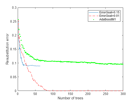
Compare the resubstitution error of the three ensembles:
figure
plot(resubLoss(rb1,'Mode','Cumulative'));
hold on
plot(resubLoss(rb2,'Mode','Cumulative'),'r--');
plot(resubLoss(ada,'Mode','Cumulative'),'g.');
hold off;
xlabel('Number of trees');
ylabel('Resubstitution error');
legend('ErrorGoal=0.15','ErrorGoal=0.01',...
    'AdaBoostM1','Location','NE');

All the RobustBoost curves show lower resubstitution error than the AdaBoostM1 curve. The error goal of 0.01 curve shows the lowest resubstitution error over most of the range.
Xtest = rand(2000,20);
Ytest = sum(Xtest(:,1:5),2) > 2.5;
idx = randsample(2000,200);
Ytest(idx) = ~Ytest(idx);
figure;
plot(loss(rb1,Xtest,Ytest,'Mode','Cumulative'));
hold on
plot(loss(rb2,Xtest,Ytest,'Mode','Cumulative'),'r--');
plot(loss(ada,Xtest,Ytest,'Mode','Cumulative'),'g.');
hold off;
xlabel('Number of trees');
ylabel('Test error');
legend('ErrorGoal=0.15','ErrorGoal=0.01',...
    'AdaBoostM1','Location','NE');

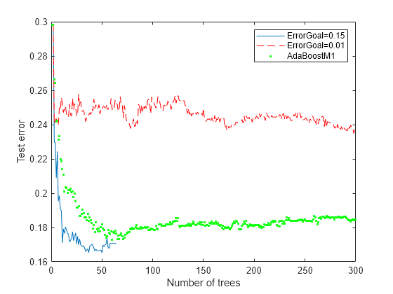
The error curve for error goal 0.15 is lowest (best) in the plotted range. AdaBoostM1 has higher error than the curve for error goal 0.15. The curve for the too-optimistic error goal 0.01 remains substantially higher (worse) than the other algorithms for most of the plotted range.
See Also
fitcensemble | resubLoss | loss