Main Content

slicesample

    Description

    rnd = slicesample(initial,nsamples,"pdf",pdf) returns a Markov chain of nsamples random samples from the density function pdf using the slice sampling method (see Algorithms). initial is a scalar or vector specifying the initial point from which the function starts sampling.

    example

    rnd = slicesample(initial,nsamples,"logpdf",logpdf) generates nsamples random samples from the log density function logpdf. During sampling, slicesample uses logpdf to evaluate the logarithm of the density function directly, instead of first evaluating the density function and then taking the log. You can use this syntax if the density function is already in logarithmic form (see Tips).

    example

    rnd = slicesample(___,Name,Value) specifies options using one or more name-value arguments in addition to any of the input argument combinations in previous syntaxes. For example, you can specify the burn-in period, the sample discard interval, and the starting interval width.

    example

    [rnd,neval] = slicesample(___) additionally returns the average number of function evaluations per sample that occurred in the slice sampling.

    example

    Examples

    collapse all

    Generate random samples from a univariate density function using slicesample.

    Create a function handle to the normal probability density function.

    rng default  % For reproducibility
    mean = 4;
    sigma = 2; % Standard deviation
    pdf = @(x) normpdf(x,mean,sigma); 

    Generate 1000 samples from pdf with no burn-in period. Use an initial value of 4.

    initial = 4;
    nsamples = 1000;
    sampleValues = slicesample(initial,nsamples,"pdf",pdf);

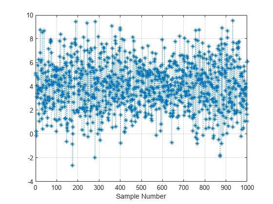
    Plot the sample value chain.

    plot(sampleValues,":*")
    grid on
    xlabel("Sample Number");

    Figure contains an axes object. The axes object with xlabel Sample Number contains an object of type line.

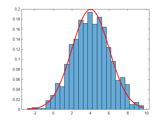
    Plot a normalized histogram of the sample values. Superimpose the normal probability density function on the histogram.

    h = histogram(sampleValues,25,"Normalization","pdf");
    hold on
    xgrid = linspace(h.BinLimits(1),h.BinLimits(2),200);
    plot(xgrid,normpdf(xgrid,mean,sigma),"r","LineWidth",2)
    hold off

    Figure contains an axes object. The axes object contains 2 objects of type histogram, line.

    The histogram shows that the resulting random samples from normpdf have an approximately normal distribution with a mean of 4 and standard deviation equal to 2.

    Generate random samples from a density function in logarithmic form using slicesample.

    Create a function handle to the logistic probability density distribution function with a mean of 0 and standard deviation equal to 1.

    pdf = @(x) exp(x)./(1+exp(x)).^2;

    Create a function handle to the loglogistic distribution function.

    logpdf = @(x) x-2*log(1+exp(x));

    Generate 1000 samples from logpdf with no burn-in period. Use an initial value of 0.

    rng default  % For reproducibility
    initial = 0;
    nsamples = 1000;
    sampleValues = slicesample(initial,nsamples,"logpdf",logpdf);

    Plot the sample value chain.

    plot(sampleValues,":*")
    grid on
    xlabel("Sample Number");

    Figure contains an axes object. The axes object with xlabel Sample Number contains an object of type line.

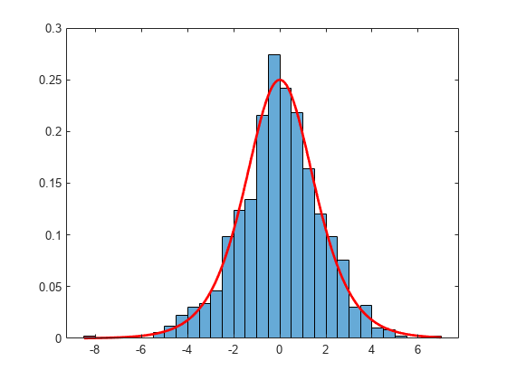
    Plot a normalized histogram of the sample values. Superimpose the logistic distribution function on the histogram.

    h = histogram(sampleValues,"Normalization","pdf");
    hold on
    xgrid = linspace(h.BinLimits(1),h.BinLimits(2),200);
    plot(xgrid,pdf(xgrid),"r","LineWidth",2)
    hold off

    Figure contains an axes object. The axes object contains 2 objects of type histogram, line.

    The histogram shows that the random samples generated from logpdf have an approximately logistic distribution.

    Generate random samples from a multimodal density function using slicesample.

    Define a function proportional to a multimodal density. The function does not need to integrate to 1.

    rng default  % For reproducibility
    pdf = @(x) exp(-x.^2/2).*(1 + (sin(3*x)).^2).* ...
        (1 + (cos(5*x).^2));

    Generate random samples from pdf, starting with an initial value of 1. Discard the first 1000 samples, and keep every fifth sample thereafter. The output sequence has 2000 samples.

    N = 2000;
    sampleValues = slicesample(1,N,"pdf",pdf,"burnin",1000,"thin",5);

    Plot a normalized histogram of the sample values. Superimpose the density function on the histogram.

    h = histogram(sampleValues,50,"Normalization","pdf");
    hold on
    xgrid = linspace(h.BinLimits(1),h.BinLimits(2),1000);
    area = integral(pdf,-5,5);
    y = pdf(xgrid)/area;
    plot(xgrid,y,"r","LineWidth",2)
    hold off

    Figure contains an axes object. The axes object contains 2 objects of type histogram, line.

    The samples provide a good fit to the multimodal density function, indicating that the specified burnin value is adequate.

    Examine the stationarity of a random sample sequence generated by slicesample, and return the average number of function evaluations per sample.

    Define a function proportional to a multimodal density.

    rng default  % For reproducibility
    pdf = @(x) exp(-x.^2/2).*(1 + (sin(3*x)).^2).* ...
        (1 + (cos(5*x).^2));

    Plot the density function.

    x = linspace(-4,4,500);
    plot(x,pdf(x),"r","LineWidth",2)
    xline(0);

    Figure contains an axes object. The axes object contains 2 objects of type line, constantline.

    The density function is symmetric about the origin and, therefore, has an expectation value of zero.

    Generate 100 samples from the density function with no burn-in period. Use an initial value of 20 and a sample width of 15.

    nsamples = 100;
    initial = 20;
    width = 15;
    burnin = 0;
    [sampleValues,neval] = slicesample(initial,nsamples, ...
        "pdf",pdf,"width",width,"burnin",burnin);
    neval
    neval = 
    4
    

    The slicesample function makes an average of neval function evaluations per generated sample.

    Plot the sample sequence values and the moving average value. Use a moving average window width of 10 samples.

    plot(sampleValues,":*")
    yline(0);
    xlabel("Sample Number");
    movavg = movmean(sampleValues,10);
    hold on
    plot(movavg,"LineWidth",2)
    hold off

    Figure contains an axes object. The axes object with xlabel Sample Number contains 3 objects of type line, constantline.

    The mean value of the sequence approaches stationarity and the expected (zero) value of the density function after approximately seven samples. You can attain stationarity faster by specifying different values for initial and burnin.

    Input Arguments

    collapse all

    Initial point to start sampling from, specified as a scalar or vector. The initial point must lie within the domain of the density function. pdf(initial) must be a strictly positive scalar. Each output sample has numel(initial) dimensions.

    Example: 1

    Data Types: single | double

    Number of output samples generated by slicesample, specified as a positive integer.

    Example: 1000

    Data Types: single | double

    Density function to generate samples from, specified as a function handle. The pdf function must accept an argument of the same type and size as initial. The pdf function can be unnormalized, meaning it does not need to integrate to 1.

    Example: @normpdf

    Data Types: function_handle

    Logarithmic density function to generate samples from, specified as a function handle. logpdf must accept an argument of the same type and size as initial. The logpdf function can be the logarithm of an unnormalized density function. During sampling, slicesample uses logpdf to evaluate the logarithm of the density function directly, instead of first evaluating the density function and then taking the log.

    Use this argument if the density function is already in logarithmic form. Doing so can improve numerical stability if logpdf has a more simple, closed form than log(pdf)(see Tips).

    Example: @(x) log(exppdf(x))

    Data Types: function_handle

    Name-Value Arguments

    Specify optional pairs of arguments as Name1=Value1,...,NameN=ValueN, where Name is the argument name and Value is the corresponding value. Name-value arguments must appear after other arguments, but the order of the pairs does not matter.

    Example: slicesample(1,4000,"pdf",pdf,burnin=1000,thin=5) generates 4000 output samples from the density function pdf, with an initial point equal to 1. The first 1000 samples are discarded, and every fifth sample is kept thereafter.

    Before R2021a, use commas to separate each name and value, and enclose Name in quotes.

    Example: slicesample(1,4000,"pdf",pdf,"burnin",1000,"thin",5) generates 4000 output samples from the density function pdf, with an initial point equal to 1. The first 1000 samples are discarded, and every fifth sample is kept thereafter.

    Number of samples to generate and discard before generating the samples to return, specified as a nonnegative integer. slicesample generates a Markov chain of samples whose stationary distribution is proportional to the density function pdf. Set burnin to a high enough value for the Markov chain to approximately reach a stationary state after generating burnin samples. For an example, see Analyze Slice Sampler Output and Performance.

    Data Types: single | double

    Sample discard interval, specified as a positive integer. slicesample discards every thin – 1 samples and keeps the next one. The slice sampling algorithm is a Markov chain, so the samples are serially correlated. To reduce the amount of serial correlation, specify a larger value for thin.

    Data Types: single | double

    Starting interval width around the current sample, specified as a nonnegative scalar or a vector of positive values. slicesample iteratively expands the interval around the current random value by width until both ends are outside the slice.

    • If width is a scalar and the samples have multiple dimensions, slicesample uses width for each dimension.

    • If width is a vector, it must have the same length as initial.

    Data Types: single | double

    Output Arguments

    collapse all

    Random sample chain, returned as an nsamples-by-numel(initial) matrix. Each row contains one sample.

    Average number of function evaluations per sample, returned as a scalar. neval includes the burnin and thin evaluations (if specified), in addition to the evaluations of samples returned in rnd. Therefore, if you specify burnin and thin values, the total number of function evaluations is neval*(nsamples*thin + burnin). Otherwise, the total number of function evaluations is neval*nsamples.

    Tips

    • Use logpdf instead of pdf for density functions where numerical overflow or underflow errors might occur.

    • There are no definitive guidelines for determining appropriate values for thin and burnin. Specify starting values for thin and burnin and then increase them, if necessary, to achieve the requisite sample independence and similarity to the target density function.

    • If the step-out procedure (see Algorithms) fails, by exceeding the maximum number of 200 function evaluations while generating a sample, you might have to experiment with different values of width. If width is too small, the algorithm might implement an excessive number of function evaluations to determine the extent of the slice. If width is too large, the algorithm tries to decrease the width to an appropriate size, which might also result in a large number of function evaluations. The neval output argument returns the average number of function evaluations per sample.

    Algorithms

    Slice sampling is a Markov Chain Monte Carlo (MCMC) algorithm that samples from a distribution with an arbitrary density function, known only up to a constant of proportionality. This situation can arise when sampling is needed from a complicated Bayesian posterior distribution whose normalization constant is unknown. The algorithm does not generate independent samples, but rather a Markov chain whose stationary distribution is the target distribution.

    The slicesample function draws samples from the region under the density function using a sequence of vertical and horizontal steps. First, the algorithm selects a height at random between 0 and the value of the density function f(x) at a specified initial value of x. Then, the algorithm selects a new x value at random by sampling from the horizontal “slice” that contains all x values where the density function is greater than the selected height. The slicesample function uses a similar slice sampling algorithm in the case of a multivariate distribution.

    Choose a density function f(x) that is proportional to the target density function, and do the following to generate a Markov chain of random numbers:

    1. Select an initial value x(t) that lies within the domain of f(x).

    2. Draw a real value y uniformly from (0, f(x(t))), thereby defining a horizontal “slice” as S = {x: y < f(x)}.

    3. Find an interval I = (L, R) around x(t) that contains all or much of the “slice” S.

    4. Draw a new point x(t + 1) from within this interval.

    5. Increment t by 1, and repeat steps 2 through 4 until you get the number of samples you want.

    slicesample uses the slice sampling algorithm of Neal[1]. For numerical stability, slicesample operates on the logarithm of the pdf function (unless the logpdf argument is specified). slicesample uses Neal's “stepping-out” and “stepping-in” method to find the interval I containing the slice S. The algorithm tries a maximum of 200 step-out and 200 step-in iterations when generating each sample.

    Nearby points in the chain tend to have values that are closer together than they would be from a sample of independent values. For many purposes, the entire set of points can be used as a sample from the target distribution. However, when this type of serial correlation is a problem, the burnin and thin name-value arguments can help reduce the correlation.

    Alternative Functionality

    • slicesample can produce Markov chains that mix slowly and take a long time to converge to a stationary distribution, especially for medium-dimensional and high-dimensional density functions. Use the gradient-based Hamiltonian Monte Carlo (HMC) sampler hmcSampler to speed up sampling in these cases. See Representing Sampling Distributions Using Markov Chain Samplers.

    References

    [1] Neal, Radford M. "Slice Sampling." The Annals of Statistics Vol. 31, No. 3, pp. 705–767, 2003. Available at https://doi.org/10.1214/aos/1056562461.

    Version History

    Introduced in R2006a