Combine Heterogeneous Models into Stacked Ensemble

Open Live Script

This example shows how to build multiple machine learning models for a given training data set, and then combine the models using a technique called stacking to improve the accuracy on a test data set compared to the accuracy of the individual models.

Stacking is a technique used to combine several heterogeneous models by training an additional model, often referred to as a stacked ensemble model, or stacked learner, on the k-fold cross-validated predictions (classification scores for classification models and predicted responses for regression models) of the original (base) models. The concept behind stacking is that certain models might correctly classify a test observation while others might fail to do so. The algorithm learns from this diversity of predictions and attempts to combine the models to improve upon the predicted accuracy of the base models.

In this example, you train several heterogeneous classification models on a data set, and then combine the models using stacking.

Load Sample Data

This example uses the 1994 census data stored in census1994.mat. The data set consists of demographic data from the US Census Bureau to predict whether an individual makes over $50,000 per year. The classification task is to fit a model that predicts the salary category of people given their age, working class, education level, marital status, race, and so on.

Load the sample data census1994 and display the variables in the data set.

load census1994
whos

  Name                 Size              Bytes  Class    Attributes

  Description         20x74               2960  char               
  adultdata        32561x15            1872567  table              
  adulttest        16281x15             944467  table

census1994 contains the training data set adultdata and the test data set adulttest. For this example, to reduce the running time, subsample 5000 training and test observations each, from the original tables adultdata and adulttest, by using the datasample function. (You can skip this step if you want to use the complete data sets.)

NumSamples = 5e3;
s = RandStream('mlfg6331_64','seed',0); % For reproducibility
adultdata = datasample(s,adultdata,NumSamples,'Replace',false);
adulttest = datasample(s,adulttest,NumSamples,'Replace',false);

Some models, such as support vector machines (SVMs), remove observations containing missing values whereas others, such as decision trees, do not remove such observations. To maintain consistency between the models, remove rows containing missing values before fitting the models.

adultdata = rmmissing(adultdata);
adulttest = rmmissing(adulttest);

Preview the first few rows of the training data set.

head(adultdata)

ans=8×15 table
    age     workClass       fnlwgt       education      education_num      marital_status         occupation         relationship     race      sex      capital_gain    capital_loss    hours_per_week    native_country    salary
    ___    ___________    __________    ____________    _____________    __________________    _________________    ______________    _____    ______    ____________    ____________    ______________    ______________    ______

    39     Private          4.91e+05    Bachelors            13          Never-married         Exec-managerial      Other-relative    Black    Male           0               0                45          United-States     <=50K 
    25     Private        2.2022e+05    11th                  7          Never-married         Handlers-cleaners    Own-child         White    Male           0               0                45          United-States     <=50K 
    24     Private        2.2761e+05    10th                  6          Divorced              Handlers-cleaners    Unmarried         White    Female         0               0                58          United-States     <=50K 
    51     Private        1.7329e+05    HS-grad               9          Divorced              Other-service        Not-in-family     White    Female         0               0                40          United-States     <=50K 
    54     Private        2.8029e+05    Some-college         10          Married-civ-spouse    Sales                Husband           White    Male           0               0                32          United-States     <=50K 
    53     Federal-gov         39643    HS-grad               9          Widowed               Exec-managerial      Not-in-family     White    Female         0               0                58          United-States     <=50K 
    52     Private             81859    HS-grad               9          Married-civ-spouse    Machine-op-inspct    Husband           White    Male           0               0                48          United-States     >50K  
    37     Private        1.2429e+05    Some-college         10          Married-civ-spouse    Adm-clerical         Husband           White    Male           0               0                50          United-States     <=50K

Each row represents the attributes of one adult, such as age, education, and occupation. The last column salary shows whether a person has a salary less than or equal to $50,000 per year or greater than $50,000 per year.

Understand Data and Choose Classification Models

Statistics and Machine Learning Toolbox™ provides several options for classification, including classification trees, discriminant analysis, naive Bayes, nearest neighbors, SVMs, and classification ensembles. For the complete list of algorithms, see Classification.

Before choosing the algorithms to use for your problem, inspect your data set. The census data has several noteworthy characteristics:

The data is tabular and contains both numeric and categorical variables.
The data contains missing values.
The response variable (salary) has two classes (binary classification).

Without making any assumptions or using prior knowledge of algorithms that you expect to work well on your data, you simply train all the algorithms that support tabular data and binary classification. Error-correcting output codes (ECOC) models are used for data with more than two classes. Discriminant analysis and nearest neighbor algorithms do not analyze data that contains both numeric and categorical variables. Therefore, the algorithms appropriate for this example are an SVM, a decision tree, an ensemble of decision trees, and a naive Bayes model.

Build Base Models

Fit two SVM models, one with a Gaussian kernel and one with a polynomial kernel. Also, fit a decision tree, a naive Bayes model, and an ensemble of decision trees.

% SVM with Gaussian kernel
rng('default') % For reproducibility
mdls{1} = fitcsvm(adultdata,'salary','KernelFunction','gaussian', ...
    'Standardize',true,'KernelScale','auto');

% SVM with polynomial kernel
rng('default')
mdls{2} = fitcsvm(adultdata,'salary','KernelFunction','polynomial', ...
    'Standardize',true,'KernelScale','auto');

% Decision tree
rng('default')
mdls{3} = fitctree(adultdata,'salary');

% Naive Bayes
rng('default')
mdls{4} = fitcnb(adultdata,'salary');

% Ensemble of decision trees
rng('default')
mdls{5} = fitcensemble(adultdata,'salary');

Combine Models Using Stacking

If you use only the prediction scores of the base models on the training data, the stacked ensemble might be subject to overfitting. To reduce overfitting, use the k-fold cross-validated scores instead. To ensure that you train each model using the same k-fold data split, create a cvpartition object and pass that object to the crossval function of each base model. This example is a binary classification problem, so you only need to consider scores for either the positive or negative class.

Obtain k-fold cross-validation scores.

rng('default') % For reproducibility
N = numel(mdls);
Scores = zeros(size(adultdata,1),N);
cv = cvpartition(adultdata.salary,"KFold",5);
for ii = 1:N
    m = crossval(mdls{ii},'cvpartition',cv);
    [~,s] = kfoldPredict(m);
    Scores(:,ii) = s(:,m.ClassNames=='<=50K');
end

Create the stacked ensemble by training it on the cross-validated classification scores Scores with these options:

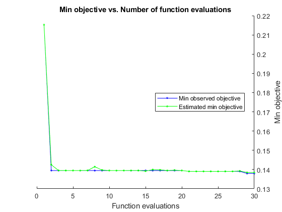
To obtain the best results for the stacked ensemble, optimize its hyperparameters. You can fit the training data set and tune parameters easily by calling the fitting function and setting its 'OptimizeHyperparameters' name-value pair argument to 'auto'.
Specify 'Verbose' as 0 to disable message displays.
For reproducibility, set the random seed and use the 'expected-improvement-plus' acquisition function. Also, for reproducibility of the random forest algorithm, specify the 'Reproducible' name-value pair argument as true for tree learners.

rng('default') % For reproducibility
t = templateTree('Reproducible',true);
stckdMdl = fitcensemble(Scores,adultdata.salary, ...
    'OptimizeHyperparameters','auto', ...
    'Learners',t, ...
    'HyperparameterOptimizationOptions',struct('Verbose',0,'AcquisitionFunctionName','expected-improvement-plus'));

Compare Predictive Accuracy

Check the classifier performance with the test data set by using the confusion matrix and McNemar's hypothesis test.

Predict Labels and Scores on Test Data

Find the predicted labels, scores, and loss values of the test data set for the base models and the stacked ensemble.

First, iterate over the base models to the compute predicted labels, scores, and loss values.

label = [];
score = zeros(size(adulttest,1),N);
mdlLoss = zeros(1,numel(mdls));
for i = 1:N
    [lbl,s] = predict(mdls{i},adulttest);
    label = [label,lbl];
    score(:,i) = s(:,m.ClassNames=='<=50K');
    mdlLoss(i) = mdls{i}.loss(adulttest);
end

Attach the predictions from the stacked ensemble to label and mdlLoss.

[lbl,s] = predict(stckdMdl,score);
label = [label,lbl];
mdlLoss(end+1) = stckdMdl.loss(score,adulttest.salary);

Concatenate the score of the stacked ensemble to the scores of the base models.

score = [score,s(:,1)];

Display the loss values.

names = {'SVM-Gaussian','SVM-Polynomial','Decision Tree','Naive Bayes', ...
    'Ensemble of Decision Trees','Stacked Ensemble'};
array2table(mdlLoss,'VariableNames',names)

ans=1×6 table
    SVM-Gaussian    SVM-Polynomial    Decision Tree    Naive Bayes    Ensemble of Decision Trees    Stacked Ensemble
    ____________    ______________    _____________    ___________    __________________________    ________________

      0.15668          0.17473           0.1975          0.16764               0.15833                  0.14519

The loss value of the stacked ensemble is lower than the loss values of the base models.

Confusion Matrix

Compute the confusion matrix with the predicted classes and the known (true) classes of the test data set by using the confusionchart function.

figure
c = cell(N+1,1);
for i = 1:numel(c)
    subplot(2,3,i)
    c{i} = confusionchart(adulttest.salary,label(:,i));
    title(names{i})
end

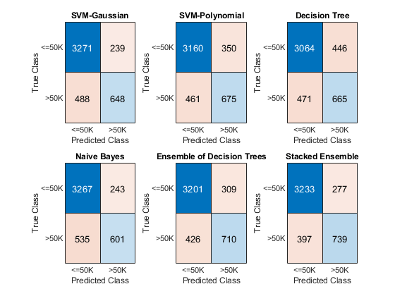
The diagonal elements indicate the number of correctly classified instances of a given class. The off-diagonal elements are instances of misclassified observations.

McNemar's Hypothesis Test

To test whether the improvement in prediction is significant, use the testcholdout function, which conducts McNemar's hypothesis test. Compare the stacked ensemble to the naive Bayes model.

 [hNB,pNB] = testcholdout(label(:,6),label(:,4),adulttest.salary)

hNB = logical
   1

pNB = 9.7646e-07

Compare the stacked ensemble to the ensemble of decision trees.

 [hE,pE] = testcholdout(label(:,6),label(:,5),adulttest.salary)

hE = logical
   1

pE = 1.9357e-04

In both cases, the low p-value of the stacked ensemble confirms that its predictions are statistically superior to those of the other models.