Edit Customizable Neural Network Using Network Editor in Classification Learner or Regression Learner
In the Classification Learner or Regression Learner app, if you have a Deep Learning Toolbox™ license, you can train neural networks with customized architecture and layer settings. This example shows how to edit a customizable neural network using the Network Editor, and then train the model and use training progress plots to check for overfitting. Although this example uses Classification Learner, you can use the same workflow in Regression Learner on a data set with a numeric response variable.
In the Command Window, load the ionosphere data set.
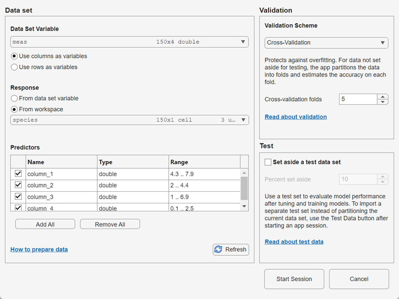
load ionosphere.matFrom the Command Window, open the Classification Learner app. Populate the New Session from Arguments dialog box with the predictor matrix
Xand the response variableY.The default validation scheme is 5-fold cross-validation, to protect against overfitting. For this example, do not change the default validation setting. To accept the selections and continue, click Start Session.classificationLearner(X,Y)
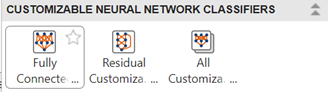
Create a customizable neural network model. In the Customizable Neural Networks section of the Models gallery, click Fully Connected Customizable Neural Network.
The Model Hyperparameters section of the model Summary tab contains training and network options. Change the number of fully connected layers to
2. The app updates the display of the network architecture.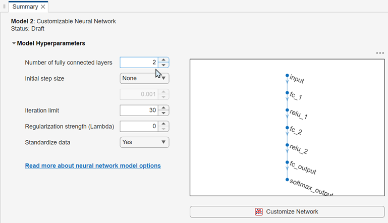
Click the Customize Network button to launch the Network Editor. You can add new layers to a network by dragging blocks from the Layer library pane into the Network pane. To quickly search for layers, use the Filter layers search box in the Layer library pane.
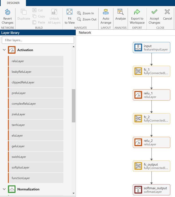
Click the first fully connected layer block (
fc_1) to display its properties. To learn more about fully connected layers, you can click the question mark icon in the Properties panel. Increase the number of activations in the first fully connected layer by changing the OutputSize value from10to15.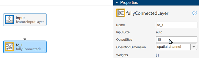
Repeat the previous step for the
fc_2block.Drag an additionLayer block from the Combination section of the Layer library pane and place it between the
fc_2andrelu_2blocks.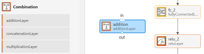
Connect the
additionblock to the network to create a skip connection. First, click the connector line between thefc_2andrelu_2blocks and press Delete. Then click the out port of thefc_2block and drag the connector line to the in port of theadditionblock.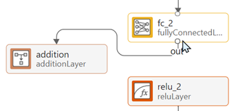
Click the out port of the
additionblock and drag the connector line to the in port of therelu_2block.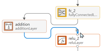
To complete the connection, click the out port of the
relu_1block and drag the connector line to the in port of theadditionblock.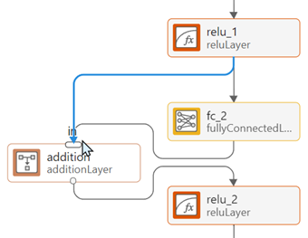
In the Close section of the Designer tab, click Accept Changes to accept your changes and close the Network Editor.
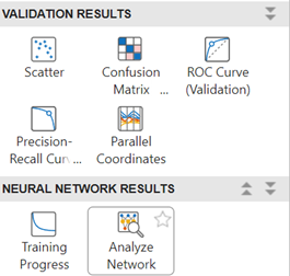
In the Neural Network Results section of the Plots and Results gallery, click Analyze Network.
The Analyze Network tab displays a network diagram and information about each layer.
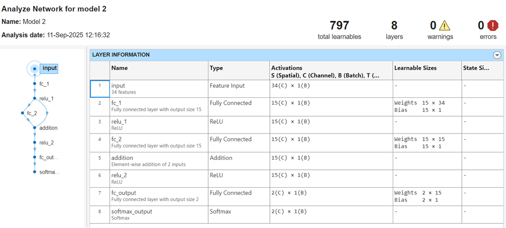
This network is a simple residual network, because it contains a skip connection between the first ReLU layer and the addition layer. Skip connections help a neural network learn residual functions (the difference between input and output). For more information about layer types, see List of Deep Learning Layers (Deep Learning Toolbox).
Train the customizable neural network model and the draft fine tree model in the Models pane. In the Train section of the Learn tab, click Train All and select Train All.
The model validation accuracy values are displayed in the Models pane.
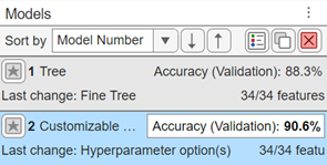
The customizable neural network model has a slightly higher validation accuracy than the fine tree model.
To view plots of training progress at each iteration for the customizable neural network model, click Training Progress in the Neural Network Results section of the Plots and Results gallery. Ensure that the Training loss, Gradient, and Step size check boxes are selected.
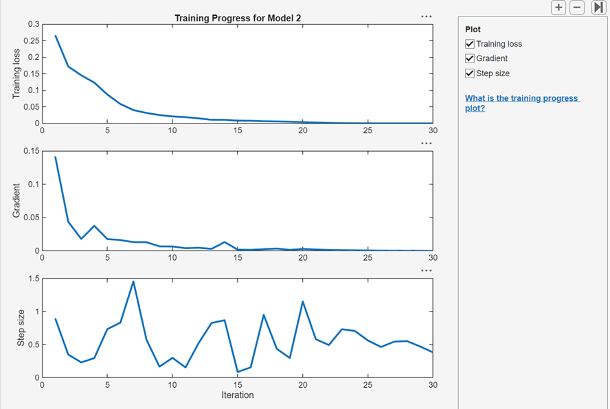
The top plot shows that the cross-entropy training loss steadily decreases with successive iterations. A flattening of the loss curve indicates that the model is approaching its optimal performance, and that further training can lead to overfitting of the data. In this example, the fitting terminates when the optimization algorithm reaches the default limit of 30 iterations. You can set the iteration limit of a draft model in the Model Hyperparameters section of the model Summary tab.
The gradient value rapidly decreases in the first few iterations and then approaches zero, indicating that the algorithm converges on optimal network learnable values. The step size fluctuates between very small values and 1.5. For more information on the optimization algorithm, see the
fitcnetreference page.