Triangular Distribution
Overview
The triangular distribution provides a simplistic representation of the probability distribution when limited sample data is available. Its parameters are the minimum, maximum, and peak of the data. Common applications include business and economic simulations, project management planning, natural phenomena modeling, and audio dithering.
Parameters
The triangular distribution uses the following parameters.
| Parameter | Description | Constraints |
|---|---|---|
a | Lower limit | |
b | Peak location | |
c | Upper limit |
The mean and variance of the triangular distribution are related to the parameters a, b, and c.
The mean is
The variance is
Parameter Estimation
Typically, you estimate triangular distribution parameters using subjectively reasonable values based on the sample data. You can estimate the lower and upper limit parameters a and c using the minimum and maximum values of the sample data, respectively. You can estimate the peak location parameter b using the sample mean, median, mode, or any other subjectively reasonable estimate of the population mode.
Probability Density Function
The probability density function (pdf) of the triangular distribution is
For an example, see Plot Triangular Distribution pdfs.
Cumulative Distribution Function
The cumulative distribution function (cdf) of the triangular distribution is
For an example, see Plot Triangular Distribution cdfs.
Examples
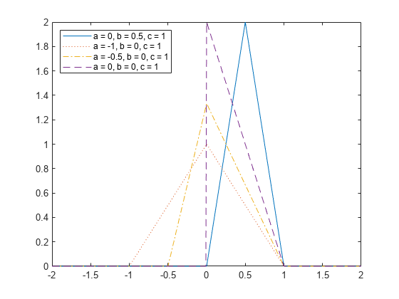
Plot Triangular Distribution pdfs
Change the value of the triangular distribution parameters a, b, and c to alter the shape of the probability distribution function (pdf).
Create four triangular distribution objects with different parameter values.
pd1 = makedist("Triangular");
pd2 = makedist("Triangular","a",-1,"b",0,"c",1);
pd3 = makedist("Triangular","a",-0.5,"b",0,"c",1);
pd4 = makedist("Triangular","a",0,"b",0,"c",1);
Compute the pdfs of the four distributions.
x = -2:0.01:2;
pdf1 = pdf(pd1,x);
pdf2 = pdf(pd2,x);
pdf3 = pdf(pd3,x);
pdf4 = pdf(pd4,x);
Plot the four pdfs.
plot(x,pdf1)
hold on
plot(x,pdf2,":")
plot(x,pdf3,"-.")
plot(x,pdf4,"--")
legend(["a = 0, b = 0.5, c = 1","a = -1, b = 0, c = 1", ...
    "a = -0.5, b = 0, c = 1","a = 0, b = 0, c = 1"], ...
    "Location","northwest");
hold off

As the distance between a and c increases, the density at any particular value within the distribution boundaries decreases. Because the density function integrates to 1, the height of the pdf plot decreases as its width increases. The location of the peak parameter b determines whether the pdf skews right or left, or if it is symmetrical.
Plot Triangular Distribution cdfs
Change the value of the triangular distribution parameters a, b, and c to alter the shape of the cumulative distribution function (cdf).
Create four triangular distribution objects with different parameters.
pd1 = makedist("Triangular");
pd2 = makedist("Triangular","a",-1,"b",0,"c",1);
pd3 = makedist("Triangular","a",-0.5,"b",0,"c",1);
pd4 = makedist("Triangular","a",0,"b",0,"c",1);
Compute the cdfs of the four distributions.
x = -1.2:0.01:1.2;
cdf1 = cdf(pd1,x);
cdf2 = cdf(pd2,x);
cdf3 = cdf(pd3,x);
cdf4 = cdf(pd4,x);
Plot the four cdfs.
plot(x,cdf1)
hold on
plot(x,cdf2,":")
plot(x,cdf3,"-.")
plot(x,cdf4,"--")
legend(["a = 0, b = 0.5, c = 1","a = -1, b = 0, c = 1", ...
    "a = -0.5, b = 0, c = 1","a = 0, b = 0, c = 1"], ...
    "Location","northwest");
xlim([-1.2 1.2]);
ylim([0 1.1])
hold off
