使用 Symbolic Math Toolbox 进行解析绘图
Symbolic Math Toolbox™ 提供数学表达式的解析绘图,而无需显式生成数值数据。这些绘图可以用二维或三维的线条、曲线、等高线、曲面或网格形式呈现。
本文中的示例介绍了以下图形函数,这些函数接受符号函数、表达式和方程作为输入:
fplotfimplicitfcontourfplot3fsurffmeshfimplicit3
使用 fplot 绘制显函数
绘制函数 。
syms x
fplot(sin(exp(x)))
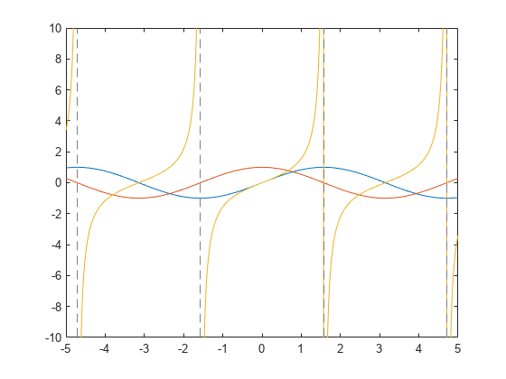
同时绘制三角函数 、 和 。
fplot([sin(x),cos(x),tan(x)])
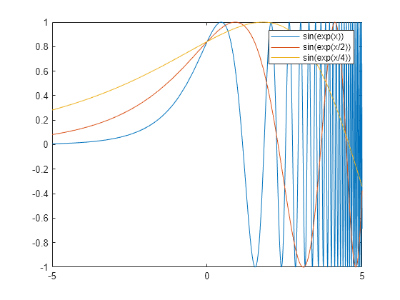
绘制由 定义的函数,其中 采用不同值
绘制函数 在 、 和 时的图。
syms x a
expr = sin(exp(x/a));
fplot(subs(expr,a,[1,2,4]))
legend show
绘制函数的导数和积分
绘制函数 、其导数 及其积分 。
syms f(x)
f(x) = x*(1 + x) + 2
f(x) =
f_diff = diff(f(x),x)
f_diff =
f_int = int(f(x),x)
f_int =
fplot([f,f_diff,f_int])
legend({'$f(x)$','$df(x)/dx$','$\int f(x)dx$'},'Interpreter','latex','FontSize',12)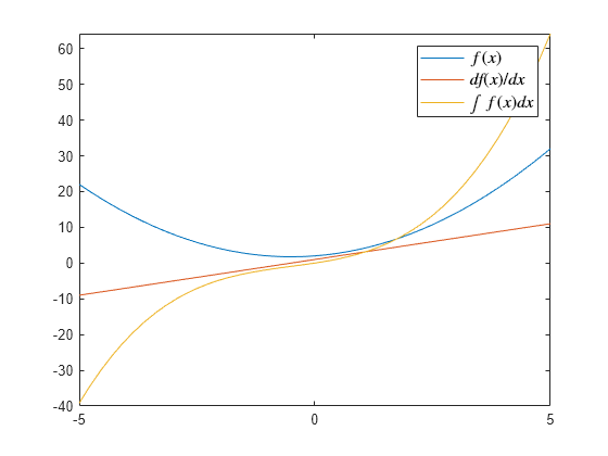
以 为水平轴绘制函数
通过求解微分方程 ,得到最小化函数 的 。
syms g(x,a);
assume(a>0);
g(x,a) = a*x*(a + x) + 2*sqrt(a)
g(x, a) =
x0 = solve(diff(g,x),x)
x0 =
绘制 的最小值,其中 的范围为 0 到 5。
fplot(g(x0,a),[0 5])
xlabel('a')
title('Minimum Value of $g(x_0,a)$ Depending on $a$','interpreter','latex')

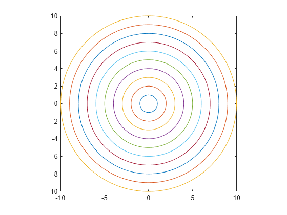
使用 fimplicit 绘制隐函数
绘制由 定义的圆,其中半径 为 1 到 10 之间的整数。
syms x y
r = 1:10;
fimplicit(x^2 + y^2 == r.^2,[-10 10])
axis square;
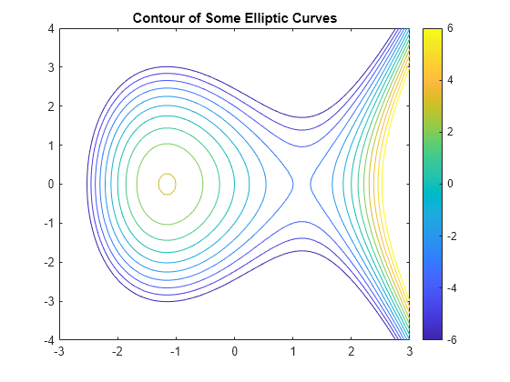
使用 fcontour 绘制函数 的等高线
针对 –6 到 6 之间的等高线层级,绘制函数 的等高线。
syms x y f(x,y)
f(x,y) = x^3 - 4*x - y^2;
fcontour(f,[-3 3 -4 4],'LevelList',-6:6);
colorbar
title 'Contour of Some Elliptic Curves'
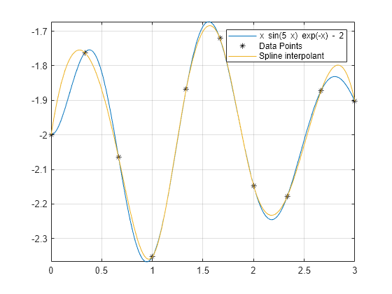
使用样条插值绘制解析函数及其逼近
绘制解析函数 。
syms f(x)
f(x) = x*exp(-x)*sin(5*x) -2;
fplot(f,[0,3])
从解析函数创建几个数据点。
xs = 0:1/3:3;
ys = double(subs(f,xs));
绘制这些数据点和逼近该解析函数的样条插值。
hold on
plot(xs,ys,'*k','DisplayName','Data Points')
fplot(@(x) spline(xs,ys,x),[0 3],'DisplayName','Spline interpolant')
grid on
legend show
hold off
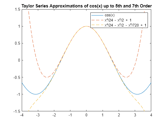
绘制函数的泰勒逼近
求 在 附近的泰勒展开式,直到 5 阶和 7 阶。
syms x
t5 = taylor(cos(x),x,'Order',5)
t5 =
t7 = taylor(cos(x),x,'Order',7)t7 =
绘制 及其泰勒逼近。
fplot(cos(x))
hold on;
fplot([t5 t7],'--')
axis([-4 4 -1.5 1.5])
title('Taylor Series Approximations of cos(x) up to 5th and 7th Order')
legend show
hold off;
绘制方波的傅里叶级数逼近
周期为 、振幅为 的方波可通过傅里叶级数展开进行逼近
绘制周期为 、振幅为 的方波。
syms t y(t)
y(t) = piecewise(0 < mod(t,2*pi) <= pi, pi/4, pi < mod(t,2*pi) <= 2*pi, -pi/4);
fplot(y)
绘制方波的傅里叶级数逼近。
hold on;
n = 6;
yFourier = cumsum(sin((1:2:2*n-1)*t)./(1:2:2*n-1));
fplot(yFourier,'LineWidth',1)
hold off

傅里叶级数逼近在跳跃间断处会出现过冲,并且随着更多项添加到逼近中,“振铃效应”不会消失。这种行为也称为吉布斯现象。
使用 fplot3 绘制参数化曲线
绘制由 定义的螺旋线,其中 的范围为 –10 到 10。
syms t
fplot3(sin(t),cos(t),t/4,[-10 10],'LineWidth',2)
view([-45 45])

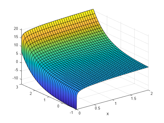
使用 fsurf 绘制由 定义的曲面
绘制由 定义的曲面。使用 fsurf 进行解析绘图(无需生成数值数据)可显示 附近的弯曲区域和渐近区域。
syms x y
fsurf(log(x) + exp(y),[0 2 -1 3])
xlabel('x')
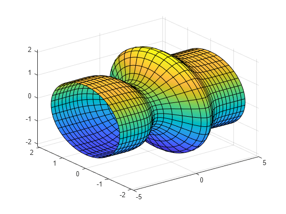
使用 fsurf 绘制多元曲面
绘制由以下各项定义的多元曲面:
其中 。
将 的绘图区间设置为 –5 到 5,并且将 的绘图区间设置为 0 到 2。
syms f(u) x(u,v) y(u,v) z(u,v)
f(u) = sin(u)*exp(-u^2/3)+1.5;
x(u,v) = u;
y(u,v) = f(u)*sin(v);
z(u,v) = f(u)*cos(v);
fsurf(x,y,z,[-5 5 0 2*pi])
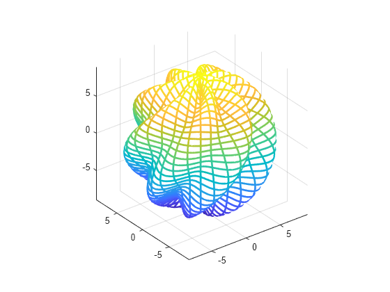
使用 fmesh 绘制多元曲面
绘制由以下各项定义的多元曲面:
其中 。使用 fmesh 将绘制的曲面显示为网格。将 的绘图区间设置为 0 到 2,并且将 的绘图区间设置为 0 到 。
syms s t
r = 8 + sin(7*s + 5*t);
x = r*cos(s)*sin(t);
y = r*sin(s)*sin(t);
z = r*cos(t);
fmesh(x,y,z,[0 2*pi 0 pi],'Linewidth',2)
axis equal
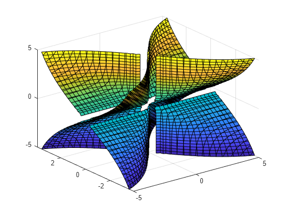
使用 fimplicit3 绘制隐式曲面
绘制隐式曲面 。
syms x y z
f = 1/x^2 - 1/y^2 + 1/z^2;
fimplicit3(f)
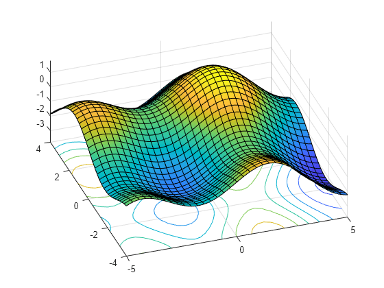
绘制曲面的等高线和梯度
使用 fsurf 绘制曲面 。您可以通过将 'ShowContours' 设置为 'on' 在同一图上显示等高线。
syms x y
f = sin(x)+sin(y)-(x^2+y^2)/20
f =
fsurf(f,'ShowContours','on')
view(-19,56)
接下来,在具有更精细等高线的单个图上绘制等高线。
fcontour(f,[-5 5 -5 5],'LevelStep',0.1,'Fill','on')
colorbar
找到曲面的梯度。使用 meshgrid 创建二维网格并代入网格坐标,以便通过数值方式计算梯度。使用 quiver 显示梯度。
hold on
Fgrad = gradient(f,[x,y])
Fgrad =
[xgrid,ygrid] = meshgrid(-5:5,-5:5);
Fx = subs(Fgrad(1),{x,y},{xgrid,ygrid});
Fy = subs(Fgrad(2),{x,y},{xgrid,ygrid});
quiver(xgrid,ygrid,Fx,Fy,'k')
hold off