Computational Mathematics in Symbolic Math Toolbox

Variables, Expressions, Functions and Equations

Variables in MATLAB® are by default double-precision. The Symbolic Math Toolbox extends this by allowing you to express numbers in exact symbolic form using sym and with variable-precision using vpa.

pi/6 + pi/4

ans = 
1.3090

sym(pi/6) + sym(pi/4)

ans = 
$$\frac{5\hspace{0.17em}\pi }{12}$$

vpa(pi/6) + vpa(pi/4)

ans = $$1.3089969389957471826927680763665$$

Symbolic variables can be used in mathematical expressions, functions and equations including trigonometric, logarithmic, exponential, and special functions. You can create symbolic expressions and perform mathematical calculations on them.

syms x y 
log(x) + exp(y)

ans = $${\mathrm{e}}^y+\log \left(x\right)$$

You can also create piecewise functions.

y(x) = piecewise(x<0, -1, x>0, 1)

y(x) = 
$$\{\begin{array}{cl}-1& \text{ if }x<0\\ 1& \text{ if }0<x\end{array}$$

Create and evaluate Create Symbolic Functions. Find the value of f at $$x=-5$$.

syms f(x)
f(x) = x^4-2*x^3+6*x^2-2*x+10

f(x) = $$x^4-2\hspace{0.17em}{x}^3+6\hspace{0.17em}{x}^2-2\hspace{0.17em}x+10$$

f(-5)

ans = $$1045$$

Find the intersection between lines $$y1$$ and $$y2$$ using solve. Equate the lines using the == operator.

syms y1 y2
y1 = x+3; y2 = 3*x;
solve(y1 == y2)

ans = 
$$\frac{3}{2}$$

Make assume on symbolic variables. There are 4 solutions to $$x^4=1$$, two real and two complex. Assuming that $$x$$ is real and $$x>0$$, there is only one solution.

syms x
solve(x^4 == 1)

ans = 
$$\left(\begin{array}{c}-1\\ 1\\ -\mathrm{i}\\ \mathrm{i}\end{array}\right)$$

assume(x,'real')
assumeAlso( x > 0)
assumptions(x)

ans = $$\left(\begin{array}{cc}x\in \mathbb{R}& 0<x\end{array}\right)$$

solve(x^4 == 1)

ans = $$1$$

assume(x,'clear')

Substitution and Solving

The Symbolic Math Toolbox supports evaluation of mathematical functions by substituting for any part of an expression using subs. You can substitute numeric values, other symbolic variables or expressions, vectors, or matrices. The Symbolic Math Toolbox supports the solving of equations and systems of equations using solve. It supports solving multivariate equations, solving inequalities and solving with assumptions. Solutions can be found symbolically or numerically with high precision by using variable-precision arithmetic.

Make substitutions with your symbolic variables. Substitute $$x=xo-1$$ into $$x^2+1$$

syms x xo
subs(x^2+1,x,xo-1)

ans = $${\left(\mathrm{xo}-1\right)}^2+1$$

Substitute multiple values. For example, evaluate $$cos(a)+sin(b)-e^{2C}$$ by substituting $$a=\frac{\pi }{2},b=\frac{\pi }{4},c=-1$$.

syms a b c
subs(cos(a) + sin(b) - exp(2*c), [a b c], [pi/2 pi/4 -1])

ans = 
$$\frac{\sqrt{2}}{2}-{\mathrm{e}}^{-2}$$

Create and solve equations. Find the zeros of $$9x^2-1=0$$.

solve(9*x^2 - 1 == 0)

ans = 
$$\left(\begin{array}{c}-\frac{1}{3}\\ \frac{1}{3}\end{array}\right)$$

Solve the general quadratic equation $$a{x}^2+bx+c=0$$ and use subs to evaluate that solution for $$a=9,b=0,c=-1$$.

eqn = a*x^2 + b*x + c == 0;
sol = solve(eqn) 

sol = 
$$\left(\begin{array}{c}-\frac{b+\sqrt{b^2-4\hspace{0.17em}a\hspace{0.17em}c}}{2\hspace{0.17em}a}\\ -\frac{b-\sqrt{b^2-4\hspace{0.17em}a\hspace{0.17em}c}}{2\hspace{0.17em}a}\end{array}\right)$$

subs(sol,[a b c],[9 0 -1])

ans = 
$$\left(\begin{array}{c}-\frac{1}{3}\\ \frac{1}{3}\end{array}\right)$$

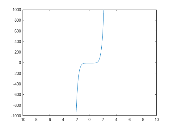
Solve equations symbolically or with variable-precision arithmetic when exact results or high precision is needed. The graph of $\mathit{f}\left(\mathit{x}\right)=6{\mathit{x}}^7-2{\mathit{x}}^6+3{\mathit{x}}^3-8$ is very flat near its root.

syms x f(x)
assume(x>0)
f(x) = 6*x^7-2*x^6+3*x^3-8;
fplot(f)
xlim([-10 10])
ylim([-1e3 1e3])

doubleSol = roots([6 -2 0 0 3 0 0 -8]) %  double-precision

doubleSol = 7×1 complex

   1.0240 + 0.0000i
   0.7652 + 0.8319i
   0.7652 - 0.8319i
  -0.8808 + 0.5043i
  -0.8808 - 0.5043i
  -0.2297 + 0.9677i
  -0.2297 - 0.9677i

symsSol = solve(f) % exact. The roots object stores the zeros for symbolic computations

symsSol = 
$$\mathrm{root}\left(z^7-\frac{z^6}{3}+\frac{z^3}{2}-\frac{4}{3},z,5\right)$$

vpaSol = vpasolve(f) % variable-precision 

vpaSol = 
$$\left(\begin{array}{c}1.0240240759053702941448316563337\\ -0.88080620051762149639205672298326+0.50434058840127584376331806592405\hspace{0.17em}\mathrm{i}\\ -0.88080620051762149639205672298326-0.50434058840127584376331806592405\hspace{0.17em}\mathrm{i}\\ -0.22974795226118163963098570610724+0.96774615576744031073999010695171\hspace{0.17em}\mathrm{i}\\ -0.22974795226118163963098570610724-0.96774615576744031073999010695171\hspace{0.17em}\mathrm{i}\\ 0.7652087814927846556172932675903+0.83187331431049713218367239317121\hspace{0.17em}\mathrm{i}\\ 0.7652087814927846556172932675903-0.83187331431049713218367239317121\hspace{0.17em}\mathrm{i}\end{array}\right)$$

Simplification and Manipulation

The Symbolic Math Toolbox supports the Formula Manipulation and Simplification of mathematical functions. Most mathematical expressions can be represented in different, but mathematically equivalent forms and the Symbolic Math Toolbox supports a number of operations, including factoring or expanding expressions, combining terms, rewriting or rearranging expressions, and simplification based on assumptions.

Perform polynomial multiplication and simplify the results, show that $$(x-1)(x+1)(x^2+x+1)(x^2+1)(x^2-x+1)(x^4-x^2+1)$$ simplifies to $$x^{12}-1$$.

simplify((x - 1)*(x + 1)*(x^2 + x + 1)*(x^2 + 1)*(x^2 - x + 1)*(x^4 - x^2 + 1))

ans = $$x^{12}-1$$

Apply trigonometric identities to simplifications, for example $$si{n}^2(x)=\frac{1-cos(2x)}{2}$$.

combine(2*sin(x)*cos(x) + (1- cos(2*x))/2 + cos(x)^2,'sincos')

ans = $$\sin \left(2\hspace{0.17em}x\right)+1$$

Factor or expand multivariate polynomials.

syms x y
factor(y^6-x^6)

ans = $$\left(\begin{array}{ccccc}-1& x-y& x+y& x^2+x\hspace{0.17em}y+y^2& x^2-x\hspace{0.17em}y+y^2\end{array}\right)$$

f(x) = (x^3 + 7);
expand(f(y-1))

ans = $$y^3-3\hspace{0.17em}{y}^2+3\hspace{0.17em}y+6$$

Find the functional composition $$f(g(x))$$.

f(x) = sqrt(log(x));
g(x) = sqrt(1-x);
h = compose(g,f,x)

h(x) = $$\sqrt{1-\sqrt{\log \left(x\right)}}$$

Calculus (Differentiation, Integration, Limits, Series, etc)

The Symbolic Math Toolbox has a full set of calculus tools for applied mathematics. It can perform multivariate symbolic integration and differentiation. It can generate, manipulate, and perform calculations with series.

Find the derivative of $$\frac{d}{dx}(\sin (x))$$.

diff(sin(x))

ans = $$\cos \left(x\right)$$

Find the derivative of $$\frac{d}{dx}(x^2+\sin (2x^4)+1)$$ using the chain rule.

diff(x^2+sin(2*x^4)+1,x)

ans = $$2\hspace{0.17em}x+8\hspace{0.17em}{x}^3\hspace{0.17em}\cos \left(2\hspace{0.17em}{x}^4\right)$$

Find the indefinite integral $$\int f(x)dx$$ for $$f(x)=e^{\frac{-x^2}{2}}$$.

int(exp(-x^2/2),x)

ans = 
$$\frac{\sqrt{2}\hspace{0.17em}\sqrt{\pi }\hspace{0.17em}\mathrm{erf}\left(\frac{\sqrt{2}\hspace{0.17em}x}{2}\right)}{2}$$

Find the definite integral $${\int }_a^{b}f(x)dx$$ for $$f(x)=x\log (1+x)$$ from $$0$$ to $$1$$.

int(x*log(1+x),0,1)

ans = 
$$\frac{1}{4}$$

Show that $$\frac{sin(x)}{x}=1$$ at $$x=0$$ by computing the Taylor series expansion $$\sum (x-a{)}^n\frac{f^{(n)}(a)}{n!}$$ for $$f(x)=\frac{sin(x)}{x}$$ around the point $$x=0$$.

syms x 
T = taylor(sin(x)/x)

T = 
$$\frac{x^4}{120}-\frac{x^2}{6}+1$$

subs(T,x,0)

ans = $$1$$

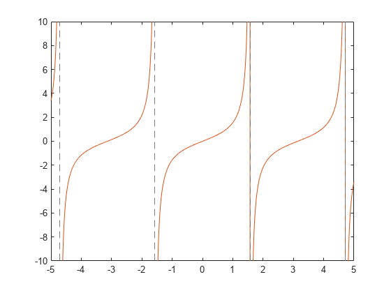
Show that $$tan(x)$$ is discontinuous at $$x=\frac{\pi }{2}$$ by showing that the left and right limits are not equal. $$\underset{x\to {\frac{\pi }{2}}^{+}}{\lim }tan(x)\ne \underset{x\to {\frac{\pi }{2}}^{-}}{\lim }tan(x)$$.

limit(tan(x),x,pi/2,'left')

ans = $$\infty$$

limit(tan(x),x,pi/2,'right')

ans = $$-\infty$$

limit(tan(x),x,pi/2)

ans = $$\mathrm{NaN}$$

Differential Equations

The Symbolic Math Toolbox can analytically solve systems of Solve a System of Differential Equations using dsolve.

Solve the first order ODE $$\frac{dy}{dx}=-ay$$.

syms a b y(x)
dsolve(diff(y) == -a*y)

ans = $$C_1\hspace{0.17em}{\mathrm{e}}^{-a\hspace{0.17em}x}$$

Solve the same ODE with the initial condition $$y(0)=b$$.

dsolve(diff(y)== -a*y,y(0)==b)

ans = $$b\hspace{0.17em}{\mathrm{e}}^{-a\hspace{0.17em}x}$$

Solve the system of coupled first order ODEs $$\frac{dx}{dt}=y$$ and $$\frac{dy}{dt}=-x$$.

syms x(t) y(t)
z = dsolve(diff(x) == y, diff(y) == -x);
disp([z.x;z.y])

$$\left(\begin{array}{c}{C}_1\hspace{0.17em}\cos \left(t\right)+C_2\hspace{0.17em}\sin \left(t\right)\\ C_2\hspace{0.17em}\cos \left(t\right)-C_1\hspace{0.17em}\sin \left(t\right)\end{array}\right)$$

Linear Algebra

The Symbolic Math Toolbox can work with symbolic vectors and matrices. It can compute eig of symbolic matrices.

Perform matrix multiplication$$Ax=b$$ where $$A=\left[\begin{array}{cc}a& b\\ c& d\end{array}\right]$$and $$x=[x1,x2]$$

syms a b c d
syms x1 x2
x = [x1; x2];
A = [a b ; c d];
b = A*x

b = 
$$\left(\begin{array}{c}a\hspace{0.17em}{x}_1+b\hspace{0.17em}{x}_2\\ c\hspace{0.17em}{x}_1+d\hspace{0.17em}{x}_2\end{array}\right)$$

Find the determinant of A.

det(A)

ans = $$a\hspace{0.17em}d-b\hspace{0.17em}c$$

Find the eigenvalues of A.

lambda = eig(A)

lambda = 
$$\left(\begin{array}{c}\frac{a}{2}+\frac{d}{2}-\frac{\sqrt{a^2-2\hspace{0.17em}a\hspace{0.17em}d+d^2+4\hspace{0.17em}b\hspace{0.17em}c}}{2}\\ \frac{a}{2}+\frac{d}{2}+\frac{\sqrt{a^2-2\hspace{0.17em}a\hspace{0.17em}d+d^2+4\hspace{0.17em}b\hspace{0.17em}c}}{2}\end{array}\right)$$

Graphics

The Symbolic Math Toolbox supports analytical plotting in 2D and 3D.

fplot(tan(x))

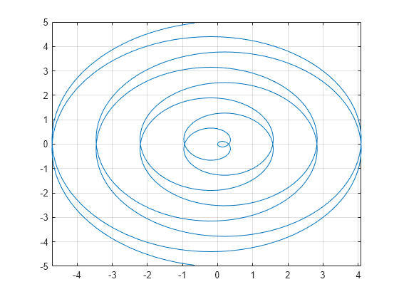
Plot the parametric curve $$x(t)=t*sin(5t)$$ and $$y(t)=t*cos(5t)$$.

syms t
x = t*sin(5*t); 
y = t*cos(5*t);
fplot(x, y)
grid on

Plot the 3D parametric curve $$x(t)=e^{\frac{|t|}{10}}sin(5|t|)$$, $$y(t)=e^{\frac{|t|}{10}}cos(5|t|)$$ and $$z(t)=t$$ from [-10,10] with a dashed red line.

syms t
xt = exp(abs(t)/10).*sin(5*abs(t));
yt = exp(abs(t)/10).*cos(5*abs(t));
zt = t;
h = fplot3(xt,yt,zt, [-10,10],'--r');

Plot the 3D surface $$f(x,y)=sin(x)+cos(y)$$.

syms x y
fsurf(sin(x) + cos(y))

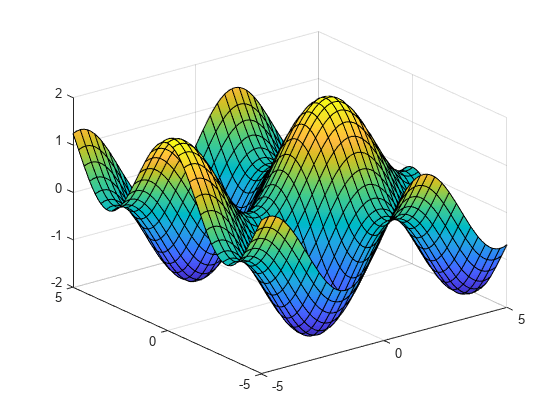
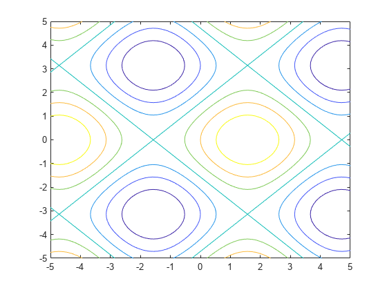
Plot the 2D contours of the same surface.

fcontour(sin(x) + cos(y))