uavCoveragePlanner

This example shows how to plan a coverage path that surveys the parking lots of the MathWorks Lakeside campus.

Get the geodetic coordinates for the MathWorks Lakeside campus. Then create the limits for our map.

mwLS = [42.3013 -71.375 0];
latlim = [mwLS(1)-0.003 mwLS(1)+0.003];
lonlim = [mwLS(2)-0.003 mwLS(2)+0.003];

Create a figure containing the map with the longitude and latitude limits.

fig = figure;
g = geoaxes(fig,Basemap="satellite");
geolimits(latlim,lonlim)

Get the outline of the first parking lot in longitude and latitude coordinates. Then create the polygon by concatenating them.

pl1lat = [42.3028 42.30325 42.3027 42.3017 42.3019]';
pl1lon = [-71.37527 -71.37442 -71.3736 -71.37378 -71.375234]';
pl1Poly = [pl1lat pl1lon];

Repeat the process for the second parking lot.

pl2lat = [42.30035 42.2999 42.2996 42.2999]';
pl2lon = [-71.3762 -71.3734 -71.37376 -71.37589]';
pl2poly = [pl2lat pl2lon];

Create the coverage space with both of those polygons, set the coverage space to use geodetic coordinates, and set the reference location to the MathWorks Lakeside campus location.

cs = uavCoverageSpace(Polygons={pl1Poly,pl2poly},UseLocalCoordinates=false,ReferenceLocation=mwLS);

Set the height at which to fly the UAV to 25 meters, and the sensor footprint width to 20 meters. Then show the coverage space on the map.

ReferenceHeight = 25;
cs.UnitWidth = 20;
show(cs,Parent=g);

Set the sweep angle for polygons 1 and 2 to 85 and 5 degrees, respectively, to have paths that are parallel to the roads in the parking lots. Then create the coverage planner for that coverage space with the exhaustive solver algorithm.

setCoveragePattern(cs,1,SweepAngle=85)
setCoveragePattern(cs,2,SweepAngle=5)
cp = uavCoveragePlanner(cs,Solver="Exhaustive");

Set the takeoff position to a location in the courtyard, then plan the coverage path.

takeoff = [42.30089 -71.3752, 0];
[wp,soln] = plan(cp,takeoff);
hold on
geoplot(wp(:,1),wp(:,2),LineWidth=1.5);
geoplot(takeoff(1),takeoff(2),MarkerSize=25,Marker=".")
legend("","","Path","Takeoff/Landing")
hold off

This example shows how to plan a coverage path for a region in local coordinates and compares the results of using the exhaustive solver with the results of using the minimum traversal solver.

Define the vertices for a coverage space.

area = [5 8.75; 5 27.5; 17.5 22.5; 25 31.25; 35 31.25; 30 20; 15 6.25];

Because vertices define a concave polygon and the coverage planner requires convex polygons, decompose the polygon into convex polygons. Then create a coverage space with the polygons from decomposition.

polygons = coverageDecomposition(area);
cs = uavCoverageSpace(Polygons=polygons);

Define the takeoff and landing positions at [0 0 0] and [32.25 37.25 0], respectively. Then show the coverage space and plot the takeoff and landing positions.

takeoff = [0 0 0];
landing = [32.25 37.25 0];
show(cs);
exampleHelperPlotTakeoffLandingLegend(takeoff,landing)

Create a coverage planner with the exhaustive solver algorithm and another coverage planner with a minimum traversal solver algorithm. Because Polygon 2 is closer to the takeoff position, set the visiting sequence of the solver parameters such that we traverse Polygon 2 first.

cpeExh = uavCoveragePlanner(cs,Solver="Exhaustive");
cpMin = uavCoveragePlanner(cs,Solver="MinTraversal");
cpeExh.SolverParameters.VisitingSequence = [2 1];
cpMin.SolverParameters.VisitingSequence = [2 1];

Plan with both solver algorithms using the same takeoff and landing positions.

[wptsExh,solnExh] = plan(cpeExh,takeoff,landing);
[wptsMin,solnMin] = plan(cpMin,takeoff,landing);

Show the planned path for both the exhaustive and the minimum traversal algorithms.

figure
show(cs);
title("Exhaustive Solver Algorithm")
exampleHelperPlotTakeoffLandingLegend(takeoff,landing,wptsExh)

figure
show(cs);
title("Minimum Traversal Solver Algorithm")
exampleHelperPlotTakeoffLandingLegend(takeoff,landing,wptsMin)

Export the waypoints from the minimum traversal solver to a .waypoints file with the reference frame set to north-east-down.

exportWaypointsPlan(cpMin,solnMin,"coveragepath.waypoints",ReferenceFrame="NED")

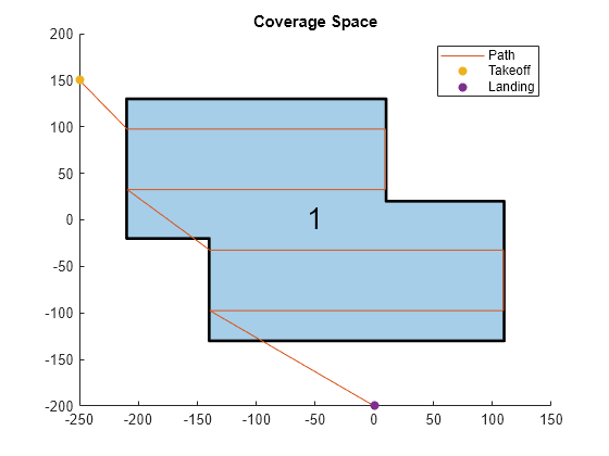
Initialize the settings to use for the coverage planner, coverage space, and mission. Set a coverage width to 65 meters, the region as polygon vertices, takeoff and landing locations, the UAV elevation during flight to 150 meters, and a geocenter.

coverageWidth = 65;
region = [-210 130; 10 130; 10 20; 110 20;
          110 -130; -140 -130; -140 -20; -210 -20];
takeoff = [-250 150 0];
landing = [0 -200 0];
uavElevation = 150;
geocenter = [-45 71 0];

Create the coverage space with those UAV coverage space settings.

cs = uavCoverageSpace(Polygons=region, ...
                      UnitWidth=coverageWidth, ...
                      ReferenceHeight=uavElevation, ...
                      ReferenceLocation=geocenter);

cs.show;
title("Coverage Space")

Create a coverage planner for the coverage space and plan the coverage path with the specified takeoff and landing locations.

cp = uavCoveragePlanner(cs);
[waypoints,solnInfo] = cp.plan(takeoff,landing);

Plot the waypoints, and the takeoff and landing locations on the coverage space.

hold on
plot(waypoints(:,1),waypoints(:,2))
scatter(takeoff(1),takeoff(2),"filled")
scatter(landing(1),landing(2),"filled")
legend("","Path","Takeoff","Landing")
hold off

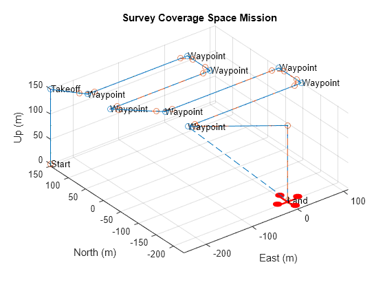
Export the waypoints to a waypoints file and create a UAV mission from that file with a speed of 10 meters per second and an initial yaw of 90 degrees.

exportWaypointsPlan(cp,solnInfo,"customCoverage.waypoints");
mission = uavMission(PlanFile="customCoverage.waypoints",Speed=10,InitialYaw=90);

Use the exampleHelperSimulateUAVMission helper function to visualize the UAV mission with a simulation time of 60 seconds.

exampleHelperSimulateUAVMission(mission,geocenter)

References

[1] Torres, Marina, David A. Pelta, José L. Verdegay, and Juan C. Torres. “Coverage Path Planning with Unmanned Aerial Vehicles for 3D Terrain Reconstruction.” Expert Systems with Applications 55 (August 2016): 441–51. https://doi.org/10.1016/j.eswa.2016.02.007.
[2] Li, Yan, Hai Chen, Meng Joo Er, and Xinmin Wang. “Coverage Path Planning for UAVs Based on Enhanced Exact Cellular Decomposition Method.” Mechatronics 21, no. 5 (August 2011): 876–85. https://doi.org/10.1016/j.mechatronics.2010.10.009.
Extended Capabilities
Generating code containing the uavCoveragePlanner requires you to enable dynamic
memory allocation. For more information about enabling dynamic memory
allocation, see Control Dynamic Memory Allocation in Generated Code (MATLAB Coder).
Deploying to embedded real time (ERT) targets is not supported.
Version History
Introduced in R2023auavCoveragePlanner now supports code generation with dynamic memory allocation
enabled. For more information about enabling dynamic memory allocation, see Control Dynamic Memory Allocation in Generated Code (MATLAB Coder).
MATLAB Command
You clicked a link that corresponds to this MATLAB command:
Run the command by entering it in the MATLAB Command Window. Web browsers do not support MATLAB commands.
选择网站
选择网站以获取翻译的可用内容,以及查看当地活动和优惠。根据您的位置,我们建议您选择:。
您也可以从以下列表中选择网站:
如何获得最佳网站性能
选择中国网站(中文或英文)以获得最佳网站性能。其他 MathWorks 国家/地区网站并未针对您所在位置的访问进行优化。
美洲
- América Latina (Español)
- Canada (English)
- United States (English)
欧洲
- Belgium (English)
- Denmark (English)
- Deutschland (Deutsch)
- España (Español)
- Finland (English)
- France (Français)
- Ireland (English)
- Italia (Italiano)
- Luxembourg (English)
- Netherlands (English)
- Norway (English)
- Österreich (Deutsch)
- Portugal (English)
- Sweden (English)
- Switzerland
- United Kingdom (English)