Generate Adversarial Examples for Semantic Segmentation

This example uses:

This example shows how to generate adversarial examples for a semantic segmentation network using the basic iterative method (BIM).

Semantic segmentation is the process of assigning each pixel in an image a class label, for example, car, bike, person, or sky. Applications for semantic segmentation include road segmentation for autonomous driving and cancer cell segmentation for medical diagnosis.

Neural networks can be susceptible to a phenomenon known as adversarial examples [1], where very small changes to an input can cause it to be misclassified. These changes are often imperceptible to humans. This example shows how to generate an adversarial example for a semantic segmentation network.

This example generates adversarial examples using the CamVid [2] data set from the University of Cambridge. The CamVid data set is a collection of images containing street-level views obtained while driving. The data set provides pixel-level labels for 32 semantic classes including car, pedestrian, and road.

Load Pretrained Network

This example loads a Deeplab v3+ network trained on the CamVid data set with weights initialized from a pretrained ResNet-18 network. For more information on building and training a Deeplab v3+ semantic segmentation network, see Semantic Segmentation Using Deep Learning (Deep Learning Toolbox).

Download a pretrained Deeplab v3+ network.

pretrainedURL = "https://www.mathworks.com/supportfiles/vision/data/deeplabv3plusResnet18CamVid_v2.zip";
pretrainedFolder = fullfile(tempdir,"pretrainedNetwork");
pretrainedNetworkZip = fullfile(pretrainedFolder,"deeplabv3plusResnet18CamVid_v2.zip"); 
if ~exist(pretrainedNetworkZip,"file")
    mkdir(pretrainedFolder);
    disp("Downloading pretrained network (58 MB)...");
    websave(pretrainedNetworkZip,pretrainedURL);
end
unzip(pretrainedNetworkZip, pretrainedFolder)

Load the network.

pretrainedNetwork = fullfile(pretrainedFolder,"deeplabv3plusResnet18CamVid_v2.mat");
data = load(pretrainedNetwork);
net = data.net;

Load Data

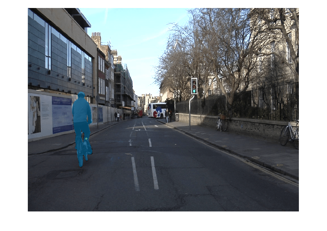
Load an image and its corresponding label image. The image is a street-level view obtained from a car being driven. The label image contains the ground truth pixel labels. In this example, you create an adversarial example that causes the semantic segmentation network to misclassify the pixels in the Bicyclist class.

img = imread("0016E5_08145.png");

Use the supporting function convertCamVidLabelImage, defined at the end of this example, to convert the label image to a categorical array.

T = convertCamVidLabelImage(imread("0016E5_08145_L.png"));

The data set contains 32 classes. Use the supporting function camVidClassNames11, defined at the end of this example, to reduce the number of classes to 11 by grouping multiple classes from the original data set together.

classNames = camVidClassNames11;

Use the supporting function camVidColorMap11 to create a colormap for the 11 classes.

cmap = camVidColorMap11;

Display the image with an overlay showing the pixels with the ground truth label Bicyclist.

classOfInterest = "Bicyclist";
notTheClassOfInterest = T ~= classOfInterest;

TClassOfInterest = T;
TClassOfInterest(notTheClassOfInterest) = "";

overlayImage = labeloverlay(img,TClassOfInterest,ColorMap=cmap);
imshow(overlayImage)

Figure contains an axes object. The axes object contains an object of type image.

Prepare Data

Create Adversarial Target Labels

To create an adversarial example, you must specify the adversarial target label for each pixel you want the network to misclassify. In this example, the aim is to get the network to misclassify the Bicyclist pixels as another class. Therefore, you need to specify target classes for each of the Bicyclist pixels.

Using the supporting function eraseClass, defined at the end of this example, create adversarial target labels by replacing all Bicyclist pixel labels with the label of the nearest pixel that is not in the Bicyclist class [3].

TDesired = eraseClass(T,classOfInterest);

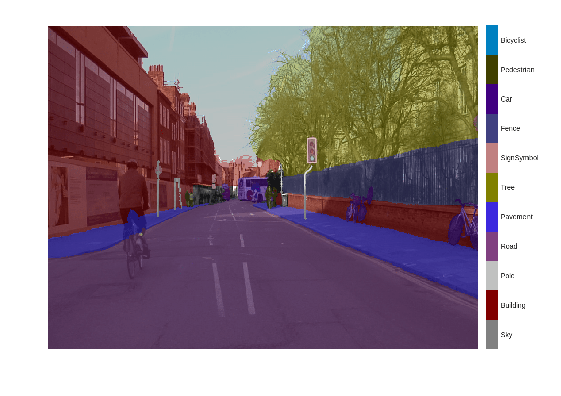
Display the adversarial target labels.

overlayImage = labeloverlay(img,TDesired,ColorMap=cmap);
figure
imshow(overlayImage)
pixelLabelColorbar(cmap,classNames);

Figure contains an axes object. The axes object contains an object of type image.

The labels of the Bicyclist pixels are now Road, Building, or Pavement.

Format Data

To create the adversarial example using the image and the adversarial target labels, you must first prepare the image and the labels.

Prepare the image by converting it to a dlarray.

X = dlarray(single(img), "SSCB");

Prepare the label by one-hot encoding it. Because some of the pixels have undefined labels, replace NaN values with 0.

TDesired = onehotencode(TDesired,3,"single",ClassNames=classNames);
TDesired(isnan(TDesired)) = 0;
TDesired = dlarray(TDesired,"SSCB");

Create Adversarial Example

Use the adversarial target labels to create an adversarial example using the basic iterative method (BIM) [4]. The BIM iteratively calculates the gradient $\nabla_{X} L (X, T)$ of the loss function $L$ with respect to the image $X$ you want to find an adversarial example for and the adversarial target labels $T$ . The negative of this gradient describes the direction to "push" the image in to make the output closer to the desired class labels.

The adversarial example image is calculated iteratively as follows:

$X_{adv} = X - α . sign (\nabla_{X} L (X, T))$ .

Parameter $α$ controls the size of the push for a single iteration. After each iteration, clip the perturbation to ensure the magnitude does not exceed $ϵ$ . Parameter $ϵ$ defines a ceiling on how large the total change can be over all the iterations. A larger $ϵ$ value increases the chance of generating a misclassified image, but makes the change in the image more visible.

Set the epsilon value to 5, set the step size alpha to 1, and perform 10 iterations.

epsilon = 5;
alpha = 1;
numIterations = 10;

Keep track of the perturbation and clip any values that exceed epsilon.

delta = zeros(size(X),like=X);
for i = 1:numIterations
    gradient = dlfeval(@targetedGradients,net,X+delta,TDesired);
    
    delta = delta - alpha*sign(gradient);
    delta(delta > epsilon) = epsilon;
    delta(delta < -epsilon) = -epsilon;
end

XAdvTarget = X + delta;

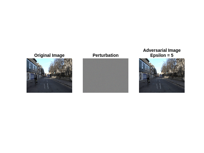
Display the original image, the perturbation added to the image, and the adversarial image.

showAdversarialImage(X,XAdvTarget,epsilon)

Figure contains 3 axes objects. Axes object 1 with title Original Image contains an object of type image. Axes object 2 with title Perturbation contains an object of type image. Axes object 3 with title Adversarial Image Epsilon = 5 contains an object of type image.

The added perturbation is imperceptible, demonstrating how adversarial examples can exploit robustness issues within a network.

Predict Pixel Labels

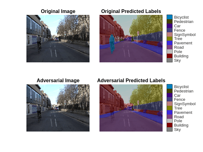
Predict the class labels of the original image and the adversarial image using the semantic segmentation network.

Y = semanticseg(extractdata(X),net);
YAdv = semanticseg(extractdata(XAdvTarget),net);

Display an overlay of the predictions for both images.

overlayImage = labeloverlay(uint8(extractdata(X)),Y,ColorMap=cmap);
overlayAdvImage = labeloverlay(uint8(extractdata(XAdvTarget)),YAdv,ColorMap=cmap);

figure
tiledlayout("flow",TileSpacing="tight")
nexttile
imshow(uint8(extractdata(X)))
title("Original Image")
nexttile
imshow(overlayImage)
pixelLabelColorbar(cmap,classNames);
title("Original Predicted Labels")
nexttile 
imshow(uint8(extractdata(XAdvTarget)))
title("Adversarial Image")
nexttile
imshow(overlayAdvImage)
pixelLabelColorbar(cmap,classNames);
title("Adversarial Predicted Labels")

Figure contains 4 axes objects. Axes object 1 with title Original Image contains an object of type image. Axes object 2 with title Original Predicted Labels contains an object of type image. Axes object 3 with title Adversarial Image contains an object of type image. Axes object 4 with title Adversarial Predicted Labels contains an object of type image.

The network correctly identifies the bicyclist in the original image. However, because of imperceptible perturbation, the network mislabels the bicyclist in the adversarial image.

Supporting Functions

convertCamVidLabelImage

The supporting function convertCamVidLabelImage takes as input a label image from the CamVid data set and converts it to a categorical array.

function labelImage = convertCamVidLabelImage(image)

colorMap32 = camVidColorMap32;
map32To11 = cellfun(@(x,y)repmat(x,size(y,1),1), ...
    num2cell((1:numel(colorMap32))'), ...
    colorMap32, ...
    UniformOutput=false);

colorMap32 = cat(1,colorMap32{:});
map32To11 = cat(1,map32To11{:});

labelImage = rgb2ind(double(image)./255,colorMap32);
labelImage = map32To11(labelImage+1);
labelImage = categorical(labelImage,1:11,camVidClassNames11);

end

camVidColorMap32

The supporting function camVidColorMap32 returns the color map for the 32 original classes in the CamVid data set.

function cmap = camVidColorMap32

cmap = {

    % Sky
    [
    128 128 128
    ]
    
    % Building
    [
      0 128  64     % Bridge
    128   0   0     % Building
     64 192   0     % Wall
     64   0  64     % Tunnel
    192   0 128     % Archway
    ]

    % Pole
    [
    192 192 128     % Column_Pole
      0   0  64     % TrafficCone
    ]

    % Road
    [
    128  64 128     % Road
    128   0 192     % LaneMkgsDriv
    192   0  64     % LaneMkgsNonDriv
    ]

    % Pavement
    [
      0   0 192     % Sidewalk 
     64 192 128     % ParkingBlock
    128 128 192     % RoadShoulder
    ]

    % Tree
    [
    128 128   0     % Tree
    192 192   0     % VegetationMisc
    ]

    % SignSymbol
    [
    192 128 128     % SignSymbol
    128 128  64     % Misc_Text
      0  64  64     % TrafficLight
    ]

    % Fence
    [
     64  64 128     % Fence
    ]

    % Car
    [
     64   0 128     % Car
     64 128 192     % SUVPickupTruck
    192 128 192     % Truck_Bus
    192  64 128     % Train
    128  64  64     % OtherMoving
    ]

    % Pedestrian
    [
     64  64   0     % Pedestrian
    192 128  64     % Child
     64   0 192     % CartLuggagePram
     64 128  64     % Animal
    ]

    % Bicyclist
    [
      0 128 192     % Bicyclist
    192   0 192     % MotorcycleScooter
    ]

    % Void
    [
      0   0   0     % Void
    ]
    
    };

% Normalize between [0 1].
cmap = cellfun(@(x)x./255,cmap,UniformOutput=false);

end

camVidColorMap11

The supporting function camVidColorMap11 returns the color map for the 11 umbrella classes in the CamVid data set.

function cmap = camVidColorMap11

cmap = [
    128 128 128     % Sky
    128   0   0     % Building
    192 192 192     % Pole
    128  64 128     % Road
     60  40 222     % Pavement
    128 128   0     % Tree
    192 128 128     % SignSymbol
     64  64 128     % Fence
     64   0 128     % Car
     64  64   0     % Pedestrian
      0 128 192     % Bicyclist
    ];

% Normalize between [0 1].
cmap = cmap ./ 255;

end

camVidClassNames11

The supporting function classNames returns the 11 umbrella classes of the CamVid data set.

function classNames = camVidClassNames11
classNames = [
    "Sky"
    "Building"
    "Pole"
    "Road"
    "Pavement"
    "Tree"
    "SignSymbol"
    "Fence"
    "Car"
    "Pedestrian"
    "Bicyclist"
    ];
end

pixelLabelColorbar

The supporting function pixelLabelColorbar adds a colorbar to the current axis. The colorbar is formatted to display the class names with the color.

function pixelLabelColorbar(cmap, classNames)
% Add a colorbar to the current axis. The colorbar is formatted
% to display the class names with the color.

colormap(gca,cmap)

% Add colorbar to current figure.
c = colorbar("peer", gca);

% Use class names for tick marks.
c.TickLabels = classNames;
numClasses = size(cmap,1);

% Center tick labels.
c.Ticks = 1/(numClasses*2):1/numClasses:1;

% Remove tick mark.
c.TickLength = 0;
end

eraseClass

The supporting function eraseClass removes class classToErase from the label image T by relabeling the pixels in class classToErase. For each pixel in class classToErase, the eraseClass function sets the pixel label to the class of the nearest pixel not in class classToErase.

function TDesired = eraseClass(T,classToErase)
classToEraseMask = T == classToErase;
[~,idx] = bwdist(~(classToEraseMask | isundefined(T)));
TDesired = T;
TDesired(classToEraseMask) = T(idx(classToEraseMask));
end

targetedGradients

Calculate the gradient used to create a targeted adversarial example. The gradient is the gradient of the mean squared error.

function gradient = targetedGradients(net,X,target)
Y = predict(net,X);
loss = mse(Y,target);
gradient = dlgradient(loss,X);
end

showAdversarialImage

Show an image, the corresponding adversarial image, and the difference between the two (perturbation).

function showAdversarialImage(image,imageAdv,epsilon)

figure
tiledlayout(1,3,TileSpacing="compact")
nexttile
imgTrue = uint8(extractdata(image));
imshow(imgTrue)
title("Original Image")

nexttile
perturbation = uint8(extractdata(imageAdv-image+127.5));
imshow(perturbation)
title("Perturbation")

nexttile
advImg = uint8(extractdata(imageAdv));
imshow(advImg)
title("Adversarial Image" + newline + "Epsilon = " + string(epsilon))
end

References

[1] Goodfellow, Ian J., Jonathon Shlens, and Christian Szegedy. “Explaining and Harnessing Adversarial Examples.” Preprint, submitted March 20, 2015. https://arxiv.org/abs/1412.6572.

[2] Brostow, Gabriel J., Julien Fauqueur, and Roberto Cipolla. “Semantic Object Classes in Video: A High-Definition Ground Truth Database.” Pattern Recognition Letters 30, no. 2 (January 2009): 88–97. https://doi.org/10.1016/j.patrec.2008.04.005.

[3] Fischer, Volker, Mummadi Chaithanya Kumar, Jan Hendrik Metzen, and Thomas Brox. “Adversarial Examples for Semantic Image Segmentation.” Preprint, submitted March 3, 2017. http://arxiv.org/abs/1703.01101.

[4] Kurakin, Alexey, Ian Goodfellow, and Samy Bengio. “Adversarial Examples in the Physical World.” Preprint, submitted February 10, 2017. https://arxiv.org/abs/1607.02533.