使用深度学习进行语义分割

此示例使用:

此示例说明如何使用语义分割网络来分割图像。

语义分割网络对图像中的每个像素进行分类，从而生成按类分割的图像。语义分割的应用包括自动驾驶中的道路分割以及医疗诊断中的癌细胞分割。要了解详细信息，请参阅Getting Started with Semantic Segmentation Using Deep Learning (Computer Vision Toolbox)。

此示例首先说明如何使用预训练的 Deeplab v3+ [1] 网络来分割图像，这是一种专门用于语义图像分割的卷积神经网络 (CNN)。其他类型的用于语义分割的网络是 U-Net。然后，您可以选择下载数据集，使用迁移学习来训练 Deeplab v3 网络。此处所示的训练过程可以应用于其他类型的语义分割网络。

为了说明训练过程，此示例使用剑桥大学的 CamVid 数据集 [2]。此数据集是包含驾驶时获得的街道级视图的图像集合。该数据集提供了 32 个语义类的像素级标签，包括汽车、行人和道路。

强烈推荐使用支持 CUDA 的 NVIDIA™ GPU 来运行此示例。使用 GPU 需要 Parallel Computing Toolbox™。有关支持的计算功能的信息，请参阅GPU Computing Requirements (Parallel Computing Toolbox)。

下载预训练的语义分割网络

下载基于 CamVid 数据集训练的 DeepLab v3+ 的预训练版本。

pretrainedURL = "https://ssd.mathworks.com/supportfiles/vision/data/deeplabv3plusResnet18CamVid_v2.zip";
pretrainedFolder = fullfile(tempdir,"pretrainedNetwork");
pretrainedNetworkZip = fullfile(pretrainedFolder,"deeplabv3plusResnet18CamVid_v2.zip"); 
if ~exist(pretrainedNetworkZip,'file')
    mkdir(pretrainedFolder);
    disp("Downloading pretrained network (58 MB)...");
    websave(pretrainedNetworkZip,pretrainedURL);
end

Downloading pretrained network (58 MB)...

unzip(pretrainedNetworkZip, pretrainedFolder)

加载该预训练网络。

pretrainedNetwork = fullfile(pretrainedFolder,"deeplabv3plusResnet18CamVid_v2.mat");  
data = load(pretrainedNetwork);
net = data.net;

设置训练此网络来进行分类所用的类。

classes = getClassNames()

classes = 11×1 string
    "Sky"
    "Building"
    "Pole"
    "Road"
    "Pavement"
    "Tree"
    "SignSymbol"
    "Fence"
    "Car"
    "Pedestrian"
    "Bicyclist"

执行语义图像分割

读取包含训练网络进行分类所用的类的图像。

I = imread("parkinglot_left.png");

将图像大小调整为网络的输入大小。

inputSize = net.Layers(1).InputSize;
I = imresize(I,inputSize(1:2));

使用 semanticseg 函数和预训练网络执行语义分割。

C = semanticseg(I,net);

使用 labeloverlay 将分割结果叠加在图像上。将叠加颜色图设置为由 CamVid 数据集 [2] 定义的颜色图值。

cmap = camvidColorMap;
B = labeloverlay(I,C,Colormap=cmap,Transparency=0.4);
figure
imshow(B)
pixelLabelColorbar(cmap, classes);

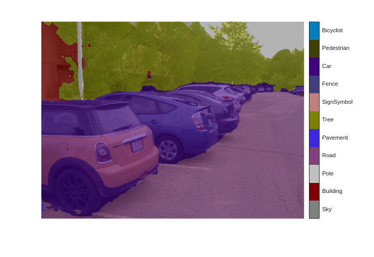
虽然网络是基于城市驾驶的图像进行预训练的，但它在停车场场景中也能生成理想的结果。为了改进分割结果，应使用包含停车场场景的其他图像来重新训练网络。此示例的其余部分说明如何使用迁移学习来训练语义分割网络。

训练语义分割网络

此示例训练的 Deeplab v3+ 网络具有从预训练的 Resnet-18 网络初始化的权重。ResNet-18 是一种高效的网络，非常适合处理资源有限的应用情形。根据应用要求，也可以使用 MobileNet v2 或 ResNet-50 等其他预训练网络。有关详细信息，请参阅预训练的深度神经网络。

使用 imagePretrainedNetwork 函数获取预训练的 ResNet-18 网络。ResNet-18 需要 Deep Learning Toolbox™ Model for ResNet-18 Network 支持包。如果未安装此支持包，则函数会提供下载链接。

imagePretrainedNetwork("resnet18")

ans = 
  dlnetwork with properties:

         Layers: [70×1 nnet.cnn.layer.Layer]
    Connections: [77×2 table]
     Learnables: [82×3 table]
          State: [40×3 table]
     InputNames: {'data'}
    OutputNames: {'prob'}
    Initialized: 1

  View summary with summary.

下载 CamVid 数据集

从以下 URL 下载 CamVid 数据集。

imageURL = "http://web4.cs.ucl.ac.uk/staff/g.brostow/MotionSegRecData/files/701_StillsRaw_full.zip";
labelURL = "http://web4.cs.ucl.ac.uk/staff/g.brostow/MotionSegRecData/data/LabeledApproved_full.zip";
 
outputFolder = fullfile(tempdir,"CamVid"); 
labelsZip = fullfile(outputFolder,"labels.zip");
imagesZip = fullfile(outputFolder,"images.zip");

if ~exist(labelsZip, 'file') || ~exist(imagesZip,'file')   
    mkdir(outputFolder)
       
    disp("Downloading 16 MB CamVid dataset labels..."); 
    websave(labelsZip, labelURL);
    unzip(labelsZip, fullfile(outputFolder,"labels"));
    
    disp("Downloading 557 MB CamVid dataset images...");  
    websave(imagesZip, imageURL);       
    unzip(imagesZip, fullfile(outputFolder,"images"));    
end

Downloading 16 MB CamVid dataset labels...

Downloading 557 MB CamVid dataset images...

注意：数据的下载时间取决于您的 Internet 连接。下载完成之前，上面使用的命令会阻止 MATLAB。您也可以使用 Web 浏览器先将数据集下载到本地磁盘。要使用从 Web 下载的文件，请将上面的 outputFolder 变量更改为下载的文件的位置。

加载 CamVid 图像

使用 imageDatastore 加载 CamVid 图像。通过 imageDatastore 可以高效加载磁盘上的大量图像。

imgDir = fullfile(outputFolder,"images","701_StillsRaw_full");
imds = imageDatastore(imgDir);

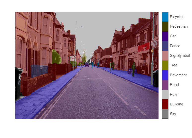
显示其中一个图像。

I = readimage(imds,559);
I = histeq(I);
imshow(I)

加载 CamVid 像素标注图像

使用 pixelLabelDatastore (Computer Vision Toolbox) 加载 CamVid 像素标签图像数据。pixelLabelDatastore 将像素标签数据和标签 ID 封装到类名映射中。

为了使训练更轻松，我们将 CamVid 中的 32 个原始类分组为 11 个类。要将 32 个类减少为 11 个，需要将原始数据集中的多个类组合在一起。例如，"Car" 是 "Car"、"SUVPickupTruck"、"Truck_Bus"、"Train" 和 "OtherMoving" 的组合。使用支持函数 camvidPixelLabelIDs 返回分组的标签 ID，该函数在此示例的末尾列出。

labelIDs = camvidPixelLabelIDs();

使用类和标签 ID 创建 pixelLabelDatastore.。

labelDir = fullfile(outputFolder,"labels");
pxds = pixelLabelDatastore(labelDir,classes,labelIDs);

读取一个像素标注图像，并将其叠加在图像上方显示。没有颜色叠加的区域没有像素标签，在训练过程中不被使用。

C = readimage(pxds,559);
cmap = camvidColorMap;
B = labeloverlay(I,C,ColorMap=cmap);
imshow(B)
pixelLabelColorbar(cmap,classes);

分析数据集统计信息

要查看 CamVid 数据集中类标签的分布，请使用 countEachLabel (Computer Vision Toolbox)。此函数按类标签计算像素数。

tbl = countEachLabel(pxds)

tbl=11×3 table
         Name         PixelCount    ImagePixelCount
    ______________    __________    _______________

    {'Sky'       }    7.6801e+07      4.8315e+08   
    {'Building'  }    1.1737e+08      4.8315e+08   
    {'Pole'      }    4.7987e+06      4.8315e+08   
    {'Road'      }    1.4054e+08      4.8453e+08   
    {'Pavement'  }    3.3614e+07      4.7209e+08   
    {'Tree'      }    5.4259e+07       4.479e+08   
    {'SignSymbol'}    5.2242e+06      4.6863e+08   
    {'Fence'     }    6.9211e+06       2.516e+08   
    {'Car'       }    2.4437e+07      4.8315e+08   
    {'Pedestrian'}    3.4029e+06      4.4444e+08   
    {'Bicyclist' }    2.5912e+06      2.6196e+08

按类可视化像素计数。

frequency = tbl.PixelCount/sum(tbl.PixelCount);

bar(1:numel(classes),frequency)
xticks(1:numel(classes)) 
xticklabels(tbl.Name)
xtickangle(45)
ylabel("Frequency")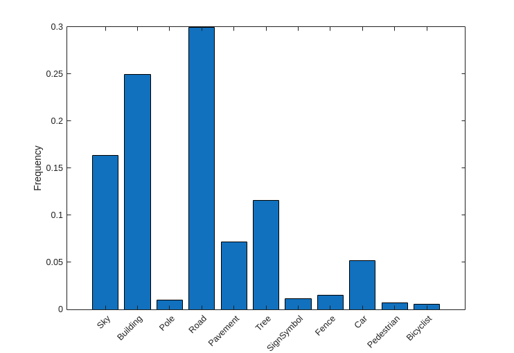

理想情况下，所有类都有相同数量的观测值。但是，CamVid 中的类是不平衡的，这是街景汽车数据集的常见问题。此类场景的天空、建筑物和道路像素比行人和骑车人像素多，因为天空、建筑物和道路覆盖了图像中的更多区域。如果处理不当，这种不平衡可能对学习过程不利，因为学习会偏向于占主导的类。在此示例的稍后部分，您将使用类权重来处理此问题。

准备训练集、验证集和测试集

使用数据集中 60% 的图像训练 Deeplab v3+。其余的图像平分成 20% 和 20%，分别用于验证和测试。以下代码将图像和像素标签数据随机分成训练集、验证集和测试集。

[imdsTrain, imdsVal, imdsTest, pxdsTrain, pxdsVal, pxdsTest] = partitionCamVidData(imds,pxds);

60/20/20 拆分将产生以下数量的训练、验证和测试图像：

numTrainingImages = numel(imdsTrain.Files)

numTrainingImages = 421

numValImages = numel(imdsVal.Files)

numValImages = 140

numTestingImages = numel(imdsTest.Files)

numTestingImages = 140

定义验证数据。

dsVal = combine(imdsVal,pxdsVal);

数据增强

数据增强可通过在训练期间随机变换原始数据来提高网络准确度。通过使用数据增强，您可以为训练数据添加更多变化，而不必增加带标签的训练样本的数量。要对图像和像素标签数据应用相同的随机变换，请使用数据存储 combine 和 transform。首先，合并 imdsTrain 和 pxdsTrain。

dsTrain = combine(imdsTrain,pxdsTrain);

接下来，使用数据存储 transform 应用在支持函数 augmentImageAndLabel 中定义的所需数据增强。此处使用随机左/右翻转和随机 X/Y 平移 +/- 10 个像素来进行数据增强。

xTrans = [-10 10];
yTrans = [-10 10];
dsTrain = transform(dsTrain, @(data)augmentImageAndLabel(data,xTrans,yTrans));

请注意，数据增强不适用于测试数据和验证数据。理想情况下，测试数据和验证数据应代表原始数据并且保持不变，以便进行无偏置的评估。

创建网络

指定网络图像大小。这通常与训练图像大小相同。

imageSize = [720 960 3];

指定类的数量。

numClasses = numel(classes);

使用 deeplabv3plus 函数基于 ResNet-18 创建一个 DeepLab v3+ 网络。为您的应用选择最佳网络需要根据经验分析，而且涉及另一级别的超参数调整。例如，您可以使用不同基础网络进行试验，如 ResNet-50 或 MobileNet v2，您也可以尝试另一个语义分割网络架构，如 U-Net。

network = deeplabv3plus(imageSize,numClasses,"resnet18");

使用类权重平衡类

如前文所示，CamVid 中的类不平衡。要改善训练，您可以使用类权重来平衡类。使用先前通过 countEachLabel (Computer Vision Toolbox) 函数计算的像素标签计数，计算具有中位数频率的类的权重。

imageFreq = tbl.PixelCount ./ tbl.ImagePixelCount;
classWeights = median(imageFreq) ./ imageFreq;

选择训练选项

用于训练的优化算法是具有动量的随机梯度下降 (SGDM)。使用 trainingOptions 指定用于 SGDM 的超参数。

学习率采用分段调度。学习率每 6 轮降低 0.1。这允许网络以更高的初始学习率快速学习，而一旦学习率下降，能够求得接近局部最优的解。

通过设置 ValidationData 名称-值参量，在每轮都对照验证数据对网络进行测试。ValidationPatience 设置为 4，以在验证准确度收敛时提前停止训练。这可以防止网络对训练数据集进行过拟合。

使用大小为 4 的小批量以减少训练时的内存使用量。您可以根据系统上的 GPU 内存量增大或减小此值。

此外，CheckpointPath 设置为临时位置。此名称-值参量让您能够在每轮训练结束时保存网络检查点。如果由于系统故障或停电而导致训练中断，您可以从保存的检查点处恢复训练。确保 CheckpointPath 指定的位置有足够的空间来存储网络检查点。例如，保存 100 个 Deeplab v3+ 检查点需要大约 6 GB 的磁盘空间，因为每个检查点大小为 61 MB。

options = trainingOptions("sgdm",...
    LearnRateSchedule="piecewise",...
    LearnRateDropPeriod=6,...
    LearnRateDropFactor=0.1,...
    Momentum=0.9,...
    InitialLearnRate=1e-2,...
    L2Regularization=0.005,...
    ValidationData=dsVal,...
    MaxEpochs=18,...  
    MiniBatchSize=4,...
    Shuffle="every-epoch",...
    CheckpointPath=tempdir,...
    VerboseFrequency=10,...
    ValidationPatience=4);

开始训练

要训练网络，请将以下代码中的 doTraining 变量设置为 true。使用 trainnet 函数训练神经网络。使用由 modelLoss 辅助函数指定的自定义损失函数。默认情况下，trainnet 函数使用 GPU（如果有）。在 GPU 上进行训练需要 Parallel Computing Toolbox™ 许可证和受支持的 GPU 设备。有关受支持设备的信息，请参阅GPU Computing Requirements (Parallel Computing Toolbox)。否则，trainnet 函数使用 CPU。要指定执行环境，请使用 ExecutionEnvironment 训练选项。

注意：该训练在具有 24 GB 内存的 NVIDIA™ GeForce RTX 3090 Ti 上进行了验证。如果您的 GPU 内存较少，则训练期间可能内存不足。如果出现这种情况，请尝试在 trainingOptions 中将 MiniBatchSize 设置为 1，或减少网络输入大小并调整训练数据的大小。训练此网络大约需要 50 分钟。根据您的 GPU 硬件情况，可能需要更长时间。

doTraining = false;
if doTraining
    [net,info] = trainnet(dsTrain,network,@(Y,T) modelLoss(Y,T,classWeights),options);
end

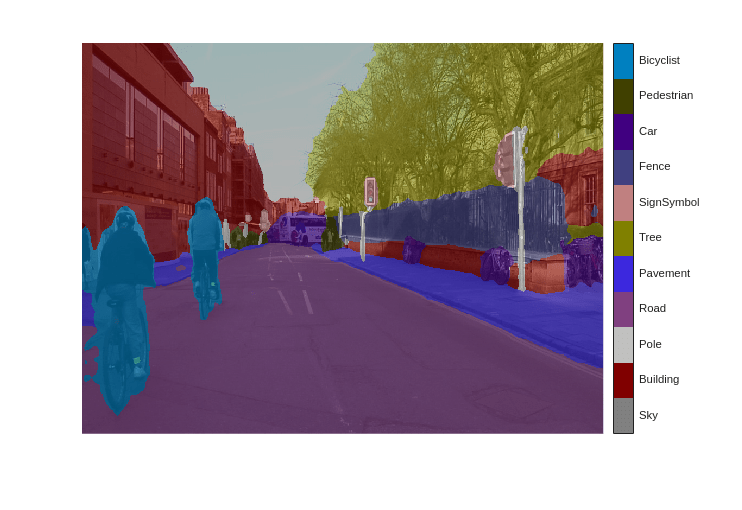
基于一个图像测试网络

在一个测试图像上运行经过训练的网络。

I = readimage(imdsTest,35);
C = semanticseg(I,net,Classes=classes);

显示结果。

B = labeloverlay(I,C,Colormap=cmap,Transparency=0.4);
imshow(B)
pixelLabelColorbar(cmap, classes);

将 C 中的结果与 pxdsTest 中存储的预期真实值进行比较。绿色和品红色区域突出显示了分割结果与预期真实值不同的区域。

expectedResult = readimage(pxdsTest,35);
actual = uint8(C);
expected = uint8(expectedResult);
imshowpair(actual, expected)

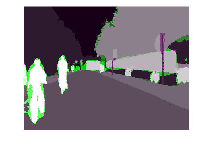
从视觉上看，语义分割结果与道路、天空、树和建筑物等类很好地重叠。然而，行人和汽车等较小的对象并不那么准确。可以使用交并比 (IoU) 度量（也称为杰卡德索引）来衡量每个类的重叠量。使用 jaccard (Image Processing Toolbox) 函数计算 IoU。

iou = jaccard(C,expectedResult);
table(classes,iou)

ans=11×2 table
      classes         iou  
    ____________    _______

    "Sky"           0.93632
    "Building"      0.87723
    "Pole"          0.40475
    "Road"          0.95332
    "Pavement"       0.8558
    "Tree"          0.92632
    "SignSymbol"    0.62978
    "Fence"         0.82389
    "Car"           0.75381
    "Pedestrian"    0.26717
    "Bicyclist"      0.7058

IoU 度量印证了可视化的结果。道路、天空、树和建筑物类具有较高的 IoU 分数，而行人和汽车等类的分数较低。其他常见的分割度量包括 dice (Image Processing Toolbox) 和 bfscore (Image Processing Toolbox) 轮廓匹配分数。

评估经过训练的网络

要衡量多个测试图像的准确度，请对整个测试集运行 semanticseg (Computer Vision Toolbox)。使用大小为 4 的小批量以减少分割图像时的内存使用量。您可以根据系统上的 GPU 内存量增大或减小此值。

pxdsResults = semanticseg(imdsTest,net, ...
    Classes=classes, ...
    MiniBatchSize=4, ...
    WriteLocation=tempdir, ...
    Verbose=false);

semanticseg 将基于测试集的结果以 pixelLabelDatastore 对象的形式返回。imdsTest 中每个测试图像的实际像素标签数据都写入到 WriteLocation 名称-值参量指定的磁盘位置。使用 evaluateSemanticSegmentation (Computer Vision Toolbox) 基于测试集结果计算各个语义分割度量。

metrics = evaluateSemanticSegmentation(pxdsResults,pxdsTest,Verbose=false);

evaluateSemanticSegmentation 返回基于整个数据集、单个类以及单个测试图像的各种度量。要查看数据集级别度量，请检查 metrics.DataSetMetrics。数据集度量提供了网络性能的高级概览。

metrics.DataSetMetrics

ans=1×5 table
    GlobalAccuracy    MeanAccuracy    MeanIoU    WeightedIoU    MeanBFScore
    ______________    ____________    _______    ___________    ___________

       0.90748          0.88828       0.69573      0.84904        0.74304

要查看每个类对整体性能的影响，请使用 metrics.ClassMetrics 检查每个类的度量。

尽管数据集整体性能非常高，但类度量显示，Pedestrian、Bicyclist 和 Car 等类表示不充分，分割效果不如 Road、Sky、Tree 和 Building 等类。增加包含更多表现不足类的样本的数据可能有助于改善结果。

metrics.ClassMetrics

ans=11×3 table
                  Accuracy      IoU      MeanBFScore
                  ________    _______    ___________

    Sky            0.9438     0.91456      0.91326  
    Building      0.84484     0.82403      0.69502  
    Pole          0.82513     0.29465      0.65171  
    Road          0.94803     0.93847      0.84376  
    Pavement      0.92135     0.77639      0.80391  
    Tree          0.89106     0.79122      0.76429  
    SignSymbol    0.81774     0.49374       0.5954  
    Fence         0.81991      0.6213      0.63421  
    Car           0.93654      0.8163       0.7784  
    Pedestrian    0.91095     0.50498      0.69317  
    Bicyclist     0.91172     0.67738      0.72119

支持函数

function labelIDs = camvidPixelLabelIDs()
% Return the label IDs corresponding to each class.
%
% The CamVid dataset has 32 classes. Group them into 11 classes following
% the original SegNet training methodology [1].
%
% The 11 classes are:
%   "Sky" "Building", "Pole", "Road", "Pavement", "Tree", "SignSymbol",
%   "Fence", "Car", "Pedestrian",  and "Bicyclist".
%
% CamVid pixel label IDs are provided as RGB color values. Group them into
% 11 classes and return them as a cell array of M-by-3 matrices. The
% original CamVid class names are listed alongside each RGB value. Note
% that the Other/Void class are excluded below.
labelIDs = { ...
    
    % "Sky"
    [
    128 128 128; ... % "Sky"
    ]
    
    % "Building" 
    [
    000 128 064; ... % "Bridge"
    128 000 000; ... % "Building"
    064 192 000; ... % "Wall"
    064 000 064; ... % "Tunnel"
    192 000 128; ... % "Archway"
    ]
    
    % "Pole"
    [
    192 192 128; ... % "Column_Pole"
    000 000 064; ... % "TrafficCone"
    ]
    
    % Road
    [
    128 064 128; ... % "Road"
    128 000 192; ... % "LaneMkgsDriv"
    192 000 064; ... % "LaneMkgsNonDriv"
    ]
    
    % "Pavement"
    [
    000 000 192; ... % "Sidewalk" 
    064 192 128; ... % "ParkingBlock"
    128 128 192; ... % "RoadShoulder"
    ]
        
    % "Tree"
    [
    128 128 000; ... % "Tree"
    192 192 000; ... % "VegetationMisc"
    ]
    
    % "SignSymbol"
    [
    192 128 128; ... % "SignSymbol"
    128 128 064; ... % "Misc_Text"
    000 064 064; ... % "TrafficLight"
    ]
    
    % "Fence"
    [
    064 064 128; ... % "Fence"
    ]
    
    % "Car"
    [
    064 000 128; ... % "Car"
    064 128 192; ... % "SUVPickupTruck"
    192 128 192; ... % "Truck_Bus"
    192 064 128; ... % "Train"
    128 064 064; ... % "OtherMoving"
    ]
    
    % "Pedestrian"
    [
    064 064 000; ... % "Pedestrian"
    192 128 064; ... % "Child"
    064 000 192; ... % "CartLuggagePram"
    064 128 064; ... % "Animal"
    ]
    
    % "Bicyclist"
    [
    000 128 192; ... % "Bicyclist"
    192 000 192; ... % "MotorcycleScooter"
    ]
    
    };
end

function classes = getClassNames()
classes = [
    "Sky"
    "Building"
    "Pole"
    "Road"
    "Pavement"
    "Tree"
    "SignSymbol"
    "Fence"
    "Car"
    "Pedestrian"
    "Bicyclist"
    ];
end

function pixelLabelColorbar(cmap, classNames)
% Add a colorbar to the current axis. The colorbar is formatted
% to display the class names with the color.

colormap(gca,cmap)

% Add colorbar to current figure.
c = colorbar('peer', gca);

% Use class names for tick marks.
c.TickLabels = classNames;
numClasses = size(cmap,1);

% Center tick labels.
c.Ticks = 1/(numClasses*2):1/numClasses:1;

% Remove tick mark.
c.TickLength = 0;
end

function cmap = camvidColorMap()
% Define the colormap used by CamVid dataset.

cmap = [
    128 128 128   % Sky
    128 0 0       % Building
    192 192 192   % Pole
    128 64 128    % Road
    60 40 222     % Pavement
    128 128 0     % Tree
    192 128 128   % SignSymbol
    64 64 128     % Fence
    64 0 128      % Car
    64 64 0       % Pedestrian
    0 128 192     % Bicyclist
    ];

% Normalize between [0 1].
cmap = cmap ./ 255;
end

function [imdsTrain, imdsVal, imdsTest, pxdsTrain, pxdsVal, pxdsTest] = partitionCamVidData(imds,pxds)
% Partition CamVid data by randomly selecting 60% of the data for training. The
% rest is used for testing.
    
% Set initial random state for example reproducibility.
rng(0); 
numFiles = numpartitions(imds);
shuffledIndices = randperm(numFiles);

% Use 60% of the images for training.
numTrain = round(0.60 * numFiles);
trainingIdx = shuffledIndices(1:numTrain);

% Use 20% of the images for validation
numVal = round(0.20 * numFiles);
valIdx = shuffledIndices(numTrain+1:numTrain+numVal);

% Use the rest for testing.
testIdx = shuffledIndices(numTrain+numVal+1:end);

% Create image datastores for training and test.
imdsTrain = subset(imds,trainingIdx);
imdsVal = subset(imds,valIdx);
imdsTest = subset(imds,testIdx);

% Create pixel label datastores for training and test.
pxdsTrain = subset(pxds,trainingIdx);
pxdsVal = subset(pxds,valIdx);
pxdsTest = subset(pxds,testIdx);
end

function data = augmentImageAndLabel(data, xTrans, yTrans)
% Augment images and pixel label images using random reflection and
% translation.

for i = 1:size(data,1)
    
    tform = randomAffine2d(...
        XReflection=true,...
        XTranslation=xTrans, ...
        YTranslation=yTrans);
    
    % Center the view at the center of image in the output space while
    % allowing translation to move the output image out of view.
    rout = affineOutputView(size(data{i,1}), tform, BoundsStyle='centerOutput');
    
    % Warp the image and pixel labels using the same transform.
    data{i,1} = imwarp(data{i,1}, tform, OutputView=rout);
    data{i,2} = imwarp(data{i,2}, tform, OutputView=rout);
    
end
end

function loss = modelLoss(Y,T,classWeights)
    weights = dlarray(classWeights,"C");
    mask = ~isnan(T);
    T(isnan(T)) = 0;
    loss = crossentropy(Y,T,weights,Mask=mask,NormalizationFactor="mask-included");
end

参考资料

[1] Chen, Liang-Chieh et al.“Encoder-Decoder with Atrous Separable Convolution for Semantic Image Segmentation.”ECCV (2018).

[2] Brostow, G. J., J. Fauqueur, and R. Cipolla."Semantic object classes in video:A high-definition ground truth database."Pattern Recognition Letters.Vol. 30, Issue 2, 2009, pp 88-97.