使用扩张卷积进行语义分割

此示例使用:

此示例说明如何使用扩张卷积训练语义分割网络。

语义分割网络对图像中的每个像素进行分类，从而生成按类分割的图像。语义分割的应用包括自动驾驶中的道路分割以及医疗诊断中的癌细胞分割。要了解详细信息，请参阅Get Started with Semantic Segmentation Using Deep Learning。

像 Deeplab v3+ [1] 这样的语义分割网络广泛使用扩张卷积（也称为空洞卷积），因为它们可以增加层的感受野（层可以看到的输入区域），而不增加参数或计算量。

加载训练数据

该示例使用 32×32 三角形图像的简单数据集进行说明。该数据集包括附带的像素标签真实值数据。使用 imageDatastore 和 pixelLabelDatastore 加载训练数据。

dataFolder = fullfile(toolboxdir("vision"),"visiondata","triangleImages");
imageFolderTrain = fullfile(dataFolder,"trainingImages");
labelFolderTrain = fullfile(dataFolder,"trainingLabels");

为图像创建一个 imageDatastore。

imdsTrain = imageDatastore(imageFolderTrain);

为真实值像素标签创建一个 pixelLabelDatastore。

classNames = ["triangle" "background"];
labels = [255 0];
pxdsTrain = pixelLabelDatastore(labelFolderTrain,classNames,labels)

pxdsTrain = 
  PixelLabelDatastore with properties:

                       Files: {200×1 cell}
                  ClassNames: {2×1 cell}
                    ReadSize: 1
                     ReadFcn: @readDatastoreImage
    AlternateFileSystemRoots: {}

创建语义分割网络

此示例使用一个基于扩张卷积的简单语义分割网络。

创建一个用于训练数据的数据源，并获取每个标签的像素计数。

ds = combine(imdsTrain,pxdsTrain);
tbl = countEachLabel(pxdsTrain)

tbl=2×3 table
         Name         PixelCount    ImagePixelCount
    ______________    __________    _______________

    {'triangle'  }         10326       2.048e+05   
    {'background'}    1.9447e+05       2.048e+05

大多数像素标签用于背景。这种类不平衡使学习过程偏向主导类。要解决此问题，请使用类权重来平衡各类。您可以使用几种方法来计算类权重。一种常见的方法是逆频率加权，其中类权重是类频率的倒数。此方法会增加指定给表示不足的类的权重。使用逆频率加权计算类权重。

numberPixels = sum(tbl.PixelCount);
frequency = tbl.PixelCount / numberPixels;
classWeights = dlarray(1 ./ frequency,"C");

使用输入大小对应于输入图像大小的图像输入层创建一个用于像素分类的网络。接下来，指定三个由卷积层、批量归一化层和 ReLU 层组成的模块。对于每个卷积层，指定 32 个具有递增扩张系数的 3×3 滤波器，并通过将 Padding 名称-值参量设置为 "same" 来填充输入以使输入的大小与输出相同。要对像素进行分类，请包括一个具有 K 个 1×1 卷积的卷积层（其中 K 是类的数量），其后是一个 softmax 层。像素的分类是是在内置训练器 trainnet 中通过一个自定义模型损失函数来完成的。

inputSize = [32 32 1];
filterSize = 3;
numFilters = 32;
numClasses = numel(classNames);

layers = [
    imageInputLayer(inputSize)
    
    convolution2dLayer(filterSize,numFilters,DilationFactor=1,Padding="same")
    batchNormalizationLayer
    reluLayer
    
    convolution2dLayer(filterSize,numFilters,DilationFactor=2,Padding="same")
    batchNormalizationLayer
    reluLayer
    
    convolution2dLayer(filterSize,numFilters,DilationFactor=4,Padding="same")
    batchNormalizationLayer
    reluLayer
    
    convolution2dLayer(1,numClasses)
    softmaxLayer];

模型损失函数

语义分割网络可以使用不同损失函数进行训练。内置训练器 trainnet (Deep Learning Toolbox) 支持自定义损失函数以及一些标准损失函数，如 crossentropy 和 mse。自定义损失函数通过将网络预测值与实际真实值或目标值进行比较来手动计算每批训练数据的损失。自定义损失函数使用函数语法为 loss = f(Y1,...,Yn,T1,...,Tm) 的函数句柄，其中 Y1,...,Yn 是对应于 n 个网络预测值的 dlarray 对象，T1,...,Tm 是对应于 m 个目标值的 dlarray 对象。

此示例使您能够从两个不同损失函数中进行选择，这两个函数说明数据中存在的类不平衡。这些损失函数是：

加权交叉熵损失，它使用 crossentropy (Deep Learning Toolbox) 函数。加权交叉熵损失通过在训练期间缩放该类的误差来对表示不充分的类提供更强的支持。
名为 tverskyLoss 的自定义损失函数，用于计算特沃斯基损失 [2]。特沃斯基损失函数更专用于处理类不平衡问题。

特沃斯基损失基于特沃斯基指数，用于衡量两个分割图像之间的重叠程度。一个图像 $Y$ 较其对应真实值 $T$ 之间的特沃斯基指数 ${TI}_{c}$ 由下式给出

${TI}_{c} = \frac{\sum_{m = 1}^{M} Y_{cm} T_{cm}}{\sum_{m = 1}^{M} Y_{cm} T_{cm} + α \sum_{m = 1}^{M} Y_{cm} T_{\overline{c} m} + β \sum_{m = 1}^{M} Y_{\overline{c} m} T_{cm}}$

$c$ 对应于类， $\overline{c}$ 对应于不在 $c$ 类中。
$M$ 是沿 $Y$ 的前两个维度的元素数量。
$α$ 和 $β$ 是控制每个类的假正和假负对损失的贡献的加权因子。

基于类数量 $C$ 的损失 $L$ 由下式给出

$L = \sum_{c = 1}^{C} 1 - {TI}_{c}$

选择训练期间要使用的损失函数。

lossFunction = "tverskyLoss"

lossFunction = 
"tverskyLoss"

if strcmp(lossFunction,"tverskyLoss")
    % Declare Tversky loss weighting coefficients for false positives and
    % false negatives. These coefficients are set and passed to the
    % training loss function using trainnet.
    alpha = 0.7;
    beta = 0.3;
    lossFcn = @(Y,T) tverskyLoss(Y,T,alpha,beta);
else
    % Use weighted cross-entropy loss during training.
    lossFcn = @(Y,T) crossentropy(Y,T,classWeights,NormalizationFactor="all-elements");
end

训练网络

指定训练选项。

options = trainingOptions("sgdm",...
    MaxEpochs=100,...
    MiniBatchSize= 64,... 
    InitialLearnRate=1e-2,...
    Verbose=false);

使用 trainnet (Deep Learning Toolbox) 训练网络。以损失函数 lossFcn 形式指定损失。

net = trainnet(ds,layers,lossFcn,options);

测试网络

加载测试数据。为图像创建一个 imageDatastore。为真实值像素标签创建一个 pixelLabelDatastore。

imageFolderTest = fullfile(dataFolder,"testImages");
imdsTest = imageDatastore(imageFolderTest);
labelFolderTest = fullfile(dataFolder,"testLabels");
pxdsTest = pixelLabelDatastore(labelFolderTest,classNames,labels);

使用测试数据和经过训练的网络进行预测。

pxdsPred = semanticseg(imdsTest,net,...
    Classes=classNames,...
    MiniBatchSize=32,...
    WriteLocation=tempdir);

Running semantic segmentation network
-------------------------------------
* Processed 100 images.

使用 evaluateSemanticSegmentation 评估预测准确度。

metrics = evaluateSemanticSegmentation(pxdsPred,pxdsTest);

Evaluating semantic segmentation results
----------------------------------------
* Selected metrics: global accuracy, class accuracy, IoU, weighted IoU, BF score.
* Processed 100 images.
* Finalizing... Done.
* Data set metrics:

    GlobalAccuracy    MeanAccuracy    MeanIoU    WeightedIoU    MeanBFScore
    ______________    ____________    _______    ___________    ___________

       0.99674          0.98562       0.96447      0.99362        0.92831

分割新图像

读取测试图像 triangleTest.jpg，并使用 semanticseg 分割测试图像。使用 labeloverlay 显示结果。

imgTest = imread("triangleTest.jpg");
[C,scores] = semanticseg(imgTest,net,classes=classNames);

B = labeloverlay(imgTest,C);
montage({imgTest,B})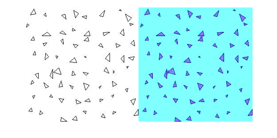

Figure contains an axes object. The axes object contains an object of type image.

支持函数

function loss = tverskyLoss(Y,T,alpha,beta)
    % loss = tverskyLoss(Y,T,alpha,beta) returns the Tversky loss
    % between the predictions Y and the training targets T.   
    
    Pcnot = 1-Y;
    Gcnot = 1-T;
    TP = sum(sum(Y.*T,1),2);
    FP = sum(sum(Y.*Gcnot,1),2);
    FN = sum(sum(Pcnot.*T,1),2); 
    
    epsilon = 1e-8;
    numer = TP + epsilon;
    denom = TP + alpha*FP + beta*FN + epsilon;
    
    % Compute tversky index.
    lossTIc = 1 - numer./denom;
    lossTI = sum(lossTIc,3);
    
    % Return average Tversky index loss.
    N = size(Y,4);
    loss = sum(lossTI)/N;
end

参考资料

[1] Chen, Liang-Chieh et al.“Encoder-Decoder with Atrous Separable Convolution for Semantic Image Segmentation.”ECCV (2018).

[2] Salehi, Seyed Sadegh Mohseni, Deniz Erdogmus, and Ali Gholipour."Tversky loss function for image segmentation using 3D fully convolutional deep networks."International Workshop on Machine Learning in Medical Imaging.Springer, Cham, 2017.