Detect Image Anomalies Using PatchCore Anomaly Detector
R2026bThis example shows how to detect and localize crack anomalies in concrete images using a PatchCore anomaly detection network.
The PatchCore model uses features extracted from convolutional neural networks (CNNs) to distinguish normal and anomalous images based on the distribution of the extracted features in feature space. The patch representation defines a mapping from the original image space to the feature space. The PatchCore model generates per-pixel and per-image anomaly scores, which you can visualize as an anomaly heatmap. The anomaly heatmap displays the probability that each pixel is anomalous, providing a visual localization of defects.
This example uses these practical advantages of the PatchCore method:
PatchCore is a one-class learning technique. You train the model using only normal (non-defective) images. Training does not require images with anomalies, which, depending on the application and industrial setting, can be rare, expensive, or unsafe to obtain.
PatchCore uses memory bank subsampling, a technique that involves dividing large image patches into smaller sub-patches and precomputing the features for each sub-patch. This technique reduces the computational cost of processing large patches during inference and improves efficiency.
PatchCore can operate in low-shot training regimes, which is an advantage for real-world visual inspection applications where access to training data consisting of normal images is limited. Sampling as little as 1% of the patch representations to be in the memory bank is sufficient for good performance and competitive inference times.
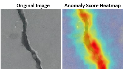
In this example, you evaluate the classification decisions of the model by inspecting correctly classified normal and anomalous images, as well as false positive and false negative images. In industrial anomaly localization applications such as this one, understanding why a trained network misclassifies certain images as anomalous is crucial.
Download Pretrained PatchCore detector
By default, this example downloads a pretrained version of the PatchCore anomaly detector using the helper function downloadTrainedNetwork. The function is attached to this example as a supporting file. You can use the pretrained network to run the entire example without waiting for training to complete.
trainedConcreteCrackDefectDetectorNet_url = "https://ssd.mathworks.com/supportfiles/visualinspection/data/trainedConcreteCrackDefectDetectorPatchCore_v1.zip";
downloadTrainedNetwork(trainedConcreteCrackDefectDetectorNet_url,pwd);
Downloading pretrained network. This can take several minutes to download... Done.
load("trainedConcreteCrackDefectDetectorPatchCore.mat");Download Concrete Crack Images for Classification Data Set
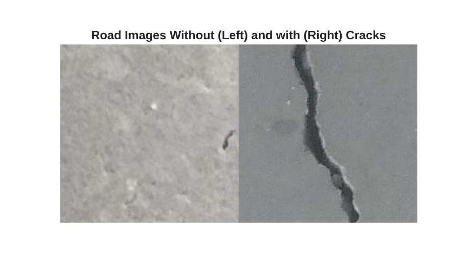
This example uses the Concrete Crack Images for Classification data set [4] [5]. The data set contains images of two classes: Negative images (or normal images) without cracks present in the road and Positive images (or anomaly images) with cracks. The data set provides 20,000 images of each class. The size of the data set is about 230 MB.
Set dataDir as the desired location of the data set.
dataDir = fullfile(tempdir,"ConcreteCrackDataset");
if ~exist(dataDir,"dir")
    mkdir(dataDir);
end
To download the data set, go to this link: https://data.mendeley.com/datasets/5y9wdsg2zt/2. Extract the ZIP file to obtain a RAR file, then extract the contents of the RAR file into the directory specified by the dataDir variable. When extracted successfully, dataDir contains two subdirectories: Negative and Positive.
Load and Preprocess Data
Create an imageDatastore that reads and manages the image data. Label each image as Positive or Negative according to the name of its directory.
imds = imageDatastore(dataDir,IncludeSubfolders=true,LabelSource="foldernames");Display an example of each class. Display a negative, or good, image without crack anomalies on the left. In the good image, imperfections and deviations in texture are small. Display a positive, or anomalous, image on the right. The anomalous image shows a large black crack oriented vertically.
positiveIdx = find(imds.Labels == "Positive", 1);
negativeIdx = find(imds.Labels == "Negative", 1);
samplePositive = readimage(imds, positiveIdx);
sampleNegative = readimage(imds, negativeIdx);
montage({sampleNegative,samplePositive})
title("Road Images Without (Left) and with (Right) Cracks")
Partition Data into Training, Calibration, and Test Sets
Define the labels for normal class and anomaly class. Normal images have the label "Negative". Anomaly images have the label "Positive" (cracks)
C = unique(imds.Labels);
normalClass = "Negative";
anomalyClasses = C(~ismember(C,normalClass));
Create training, calibration, and test sets using the splitAnomalyData function. This example uses a PatchCore network.
Allocate 250 normal images for training. Allocate 50 of each normal and anomaly images for calibration and 500 normal and 500 anomaly images to the test set. Using a smaller training set takes advantage of PatchCore's performance in low-shot training and decreases peak memory usage during training.
normalTotal = 20000;
anomalyTotal = 20000;

normalTrain = 250;
normalCal = 50;
normalTest = 500;

anomalyTrain = 0;
anomalyCal = 50;
anomalyTest = 500;

normalTrainRatio = normalTrain / normalTotal;
normalCalRatio = normalCal / normalTotal;
normalTestRatio = normalTest / normalTotal;

anomalyTrainRatio = anomalyTrain / anomalyTotal;
anomalyCalRatio = anomalyCal / anomalyTotal;
anomalyTestRatio = anomalyTest / anomalyTotal;

anomalyClasses = anomalyClasses(:)';

[imdsTrain,imdsCal,imdsTest] = splitAnomalyData(imds,anomalyClasses, ...
NormalLabelsRatio=[normalTrainRatio normalCalRatio normalTestRatio], ...
AnomalyLabelsRatio=[anomalyTrainRatio anomalyCalRatio anomalyTestRatio]);
Splitting anomaly dataset
-------------------------
* Finalizing... Done.
* Number of files and proportions per class in all the datasets:

                      Input                Train             Validation              Test
                _________________    _________________    _________________    _________________

                NumFiles    Ratio    NumFiles    Ratio    NumFiles    Ratio    NumFiles    Ratio
                ________    _____    ________    _____    ________    _____    ________    _____

    Negative     20000       0.5       250         1         50        0.5       500        0.5
    Positive     20000       0.5         0         0         50        0.5       500        0.5
Define an anonymous function, addLabelFcn, that creates a one-hot encoded representation of label information from an input image. Then, transform the datastores by using the transform function such that the datastores return a cell array of image data and a corresponding one-hot encoded array. The transform function applies the operations specified by addLabelFcn.
addLabelFcn = @(x,info) deal({x,onehotencode(info.Label,1)},info);
imdsTrain = transform(imdsTrain,addLabelFcn,IncludeInfo=true);
imdsCal = transform(imdsCal,addLabelFcn,IncludeInfo=true);
imdsTest = transform(imdsTest,addLabelFcn,IncludeInfo=true);
Resize and Crop Images
Define an anonymous function, resizeAndCropImageFcn, that applies the resizeAndCropForConcreteAnomalyDetector helper function to the input images. The resizeAndCropForConcreteAnomalyDetector helper function, which is attached to this example as a supporting file, resizes and center-crops input images. Transform the datastores by using the transform function with the operations specified by resizeAndCropImageFcn. This operation crops each image in the training, calibration, and test datastores to a size of 244-by-224 to match the input size of the pretrained CNN.
resizeImageSize = [256 256];
targetImageSize = [224 224];
resizeAndCropImageFcn = @(x,info) ...
    deal({resizeAndCropForConcreteAnomalyDetector(x{1},resizeImageSize,targetImageSize),x{2}});
imdsTrain = transform(imdsTrain,resizeAndCropImageFcn);
imdsCal = transform(imdsCal,resizeAndCropImageFcn);
imdsTest = transform(imdsTest,resizeAndCropImageFcn);
Define PatchCore Anomaly Detector Network Architecture
Set up the PatchCore detector [1] to extract mid-level features from a CNN backbone. During training, PatchCore adds these features to a memory bank, and subsamples them to compress the memory bank of feature embeddings. The backbone of PatchCore in this example is the ResNet-18 network [2], a CNN that has 18 layers and is pretrained on ImageNet [3].
Create a PatchCore anomaly detector network by using the patchCoreAnomalyDetector function with the ResNet-18 backbone.
patchCore = patchCoreAnomalyDetector(Backbone="resnet18");Train Detector
To train the detector, set the doTraining variable to true. Train the detector by using the trainPatchCoreAnomalyDetector function with the untrained PatchCore detector network, patchCore, and the training data, imdsTrain, as inputs. Specify the CompressionRatio name-value argument as 0.1, so that a small ratio of the original features, or memory bank, is preserved, and the model still shows satisfactory performance.
Train on one or more GPUs, if they are available. Using a GPU requires a Parallel Computing Toolbox™ license and a CUDA®-enabled NVIDIA® GPU. For more information, see GPU Computing Requirements (Parallel Computing Toolbox).
doTraining =false; if doTraining detector = trainPatchCoreAnomalyDetector(imdsTrain,patchCore,CompressionRatio=0.1); modelDateTime = string(datetime("now",Format="yyyy-MM-dd-HH-mm-ss")); save(string(tempdir)+filesep+"trainedConcreteCrackDetectorPatchCore_"+modelDateTime+".mat", ... "detector"); end
Set Anomaly Threshold
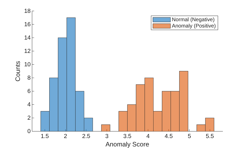
An important stage of semi-supervised anomaly detection is choosing an anomaly score threshold for separating normal images from anomalous images. This example uses a calibration data set that contains both normal and anomalous images to select the threshold.
Obtain the mean anomaly score and ground truth label for each image in the calibration set.
scores = predict(detector,imdsCal);
labels = imdsCal.UnderlyingDatastores{1}.Labels ~= "Negative";
Plot a histogram of the mean anomaly scores for the normal and anomaly classes. The distributions are well separated by the model-predicted anomaly score.
numBins = 20;
[~,edges] = histcounts(scores,numBins);
figure
hold on
hNormal = histogram(scores(labels==0),edges);
hAnomaly = histogram(scores(labels==1),edges);
hold off
legend([hNormal,hAnomaly],"Normal (Negative)","Anomaly (Positive)")
xlabel("Anomaly Score")
ylabel("Counts")
Calculate the optimal anomaly threshold by using the anomalyThreshold function. Specify the first two input arguments as the ground truth labels, labels, and predicted anomaly scores, scores, for the calibration data set. Specify the third input argument as true because true positive anomaly images have a labels value of true. The anomalyThreshold function returns the optimal threshold value as a scalar and the receiver operating characteristic (ROC) curve for the detector as an rocmetrics (Deep Learning Toolbox) object.
[thresh,roc] = anomalyThreshold(labels,scores,true,"MaxF1Score");Set the Threshold property of the anomaly detector to the optimal value.
detector.Threshold = thresh;
Plot the ROC curve by using the plot (Deep Learning Toolbox) object function of the rocmetrics object. The ROC curve illustrates the performance of the classifier for a range of possible threshold values. Each point on the ROC curve represents the false positive rate (x-coordinate) and true positive rate (y-coordinate) when the calibration set images are classified using a different threshold value. The solid blue line represents the ROC curve. The area under the ROC curve (AUC) metric indicates classifier performance, and the maximum ROC AUC corresponding to a perfect classifier is 1.0.
plot(roc)
title("ROC AUC: "+ roc.AUC)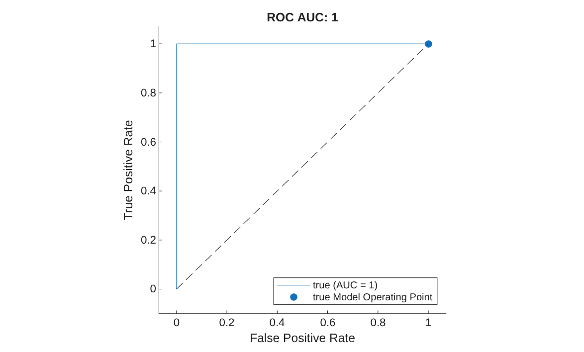
Evaluate Classification Model
Classify Test Images
Classify each image in the test set as either normal or anomalous by using the classify function. The function compares the anomaly score of each image to the threshold value stored in detector.
testSetOutputLabels = classify(detector,imdsTest);
testSetOutputLabels = testSetOutputLabels';
Get the ground truth labels of each test image
testSetTargetLabels = imdsTest.UnderlyingDatastores{1}.Labels;Evaluate the anomaly detector by calculating performance metrics using the evaluateAnomalyDetection function. The function calculates several metrics that evaluate the accuracy, precision, sensitivity, and specificity of the detector for the test data set.
metrics = evaluateAnomalyDetection(testSetOutputLabels,testSetTargetLabels,"Positive");Evaluating anomaly detection results
------------------------------------
* Finalizing... Done.
* Data set metrics:
GlobalAccuracy MeanAccuracy Precision Recall Specificity F1Score FalsePositiveRate FalseNegativeRate
______________ ____________ _________ ______ ___________ _______ _________________ _________________
0.99 0.99 0.99395 0.986 0.994 0.98996 0.006 0.014
The ConfusionMatrix property of metrics contains the confusion matrix for the test set. Extract the confusion matrix and display a confusion plot. The classification model in this example is very accurate and predicts a small percentage of false positives and false negatives.
M = metrics.ConfusionMatrix{:,:};
confusionchart(M,["Negative","Positive"])
acc = sum(diag(M)) / sum(M,"all");
title("Accuracy: "+acc);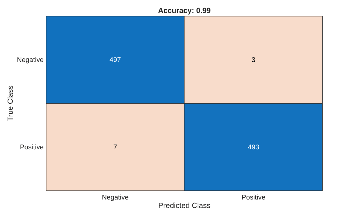
Explain Classification Decisions
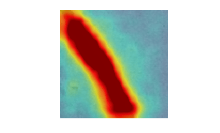
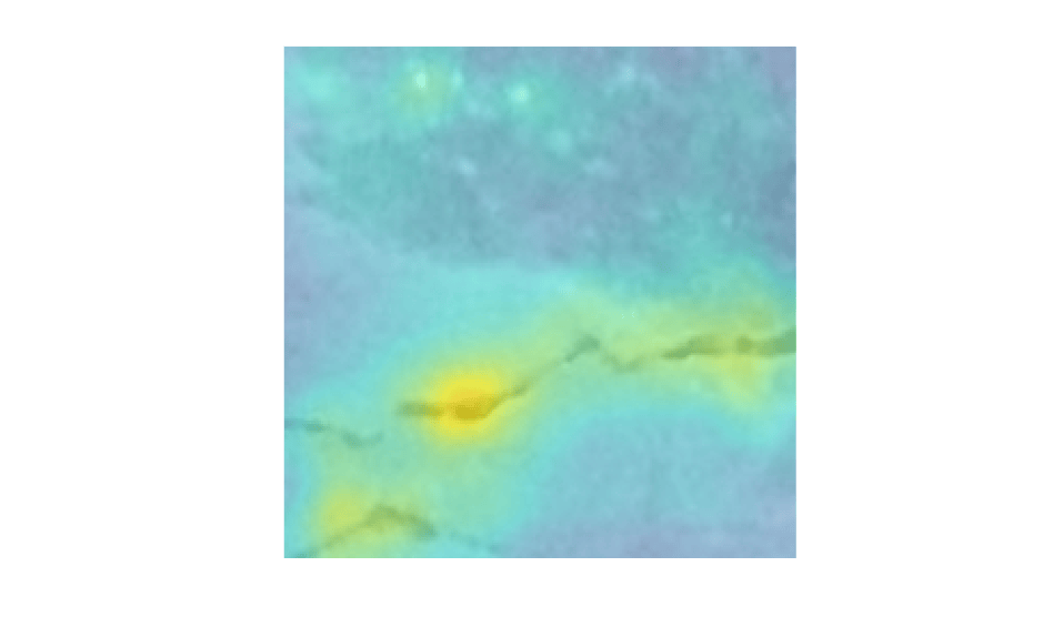
You can visualize the anomaly score map predicted by the PatchCore detector as a heatmap overlaid on the image. You can use this localization of predicted anomalies to help explain why an image is classified as normal or anomalous. This approach is useful for identifying patterns in false negatives and false positives. You can use these patterns to identify strategies to improve the network performance.
Calculate Anomaly Heatmap Display Range
Calculate a display range that reflects the range of anomaly score values observed in the calibration set, including normal and anomalous images. By using the same display range across images, you can compare images more easily than if you scale each image to its own minimum and maximum. Use the anomalyMap function to generate the anomaly score map for each image in the calibration set, and track the global minimum and maximum score values. Then, define a common display range from the global minimum to 70% of the global maximum to improve visual contrast.
minMapVal = inf;
maxMapVal = -inf;
reset(imdsCal)
while hasdata(imdsCal)
    img = read(imdsCal);
    map = anomalyMap(detector,img{1});
    minMapVal = min(min(map,[],"all"),minMapVal);
    maxMapVal = max(max(map,[],"all"),maxMapVal);
end
displayRange = [minMapVal 0.7*maxMapVal];
View Heatmap of Anomaly
Select an image of a correctly classified anomaly. Display the image with the heatmap overlay by using anomalyMapOverlay function.
testSetAnomalyLabels = testSetTargetLabels ~= "Negative";
idxTruePositive = find(testSetAnomalyLabels & testSetOutputLabels,1);
dsExample = subset(imdsTest,idxTruePositive);
data = read(dsExample);
img = data{1};
map = anomalyMap(detector,img);
imshow(anomalyMapOverlay(img,map,MapRange=displayRange,Blend="proportional"))
View Heatmap of Normal Image
Select and display an image of a correctly classified normal image. This result is a true negative classification.
idxTrueNegative = find(~(testSetAnomalyLabels | testSetOutputLabels));
dsExample = subset(imdsTest,idxTrueNegative);
data = read(dsExample);
img = data{1};
map = anomalyMap(detector,img);
imshow(anomalyMapOverlay(img,map,MapRange=displayRange,Blend="proportional"))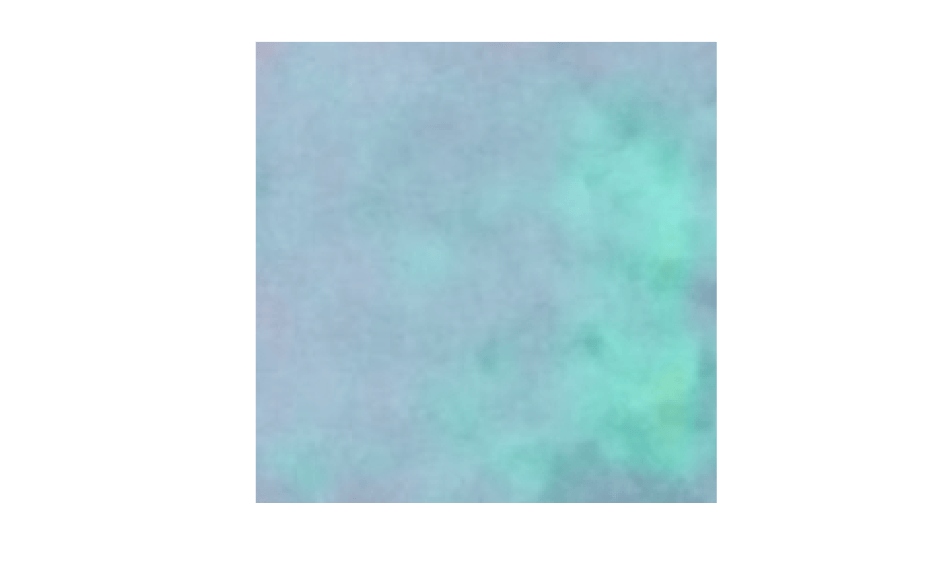
View Heatmap of False Positive Images
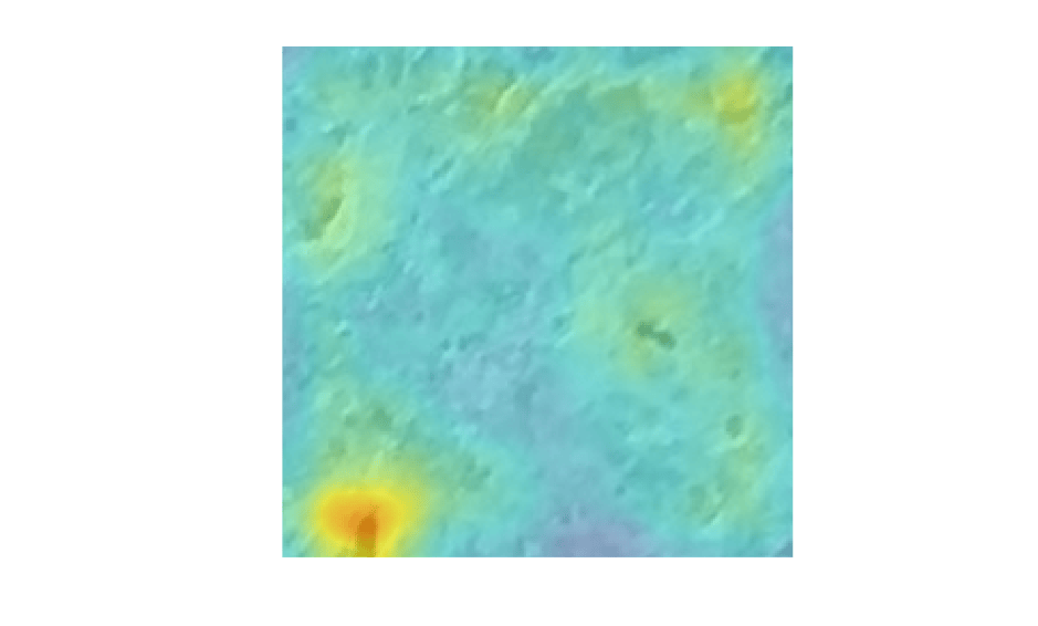
False positives are images without crack anomalies that the network classifies as anomalous. Use the anomaly heatmap to gain insight into the misclassifications.
Find false positive images from the test set. Display three false positive images as a montage.
idxFalsePositive = find(~testSetAnomalyLabels & testSetOutputLabels);
if ~isempty(idxFalsePositive)
    dsExample = subset(imdsTest, idxFalsePositive);
    data = read(dsExample);
    img = data{1};
    map = anomalyMap(detector, img);
figure;
imshow(anomalyMapOverlay(img,map,MapRange=displayRange,Blend="proportional"));
end
View Heatmap of False Negative Images
False negatives are images with crack anomalies that the network classifies as normal.
Find any false negative images from the test set. Display three false negative images as a montage.
idxFalseNegative = find(testSetAnomalyLabels & (~testSetOutputLabels));
if ~isempty(idxFalseNegative)
    dsExample = subset(imdsTest, idxFalseNegative);
    data = read(dsExample);
    img = data{1};
    map = anomalyMap(detector, img);
figure;
imshow(anomalyMapOverlay(img,map,MapRange=displayRange,Blend="proportional"));
end
References
[1] Roth, Karsten, Latha Pemula, Joaquin Zepeda, Bernhard Schölkopf, Thomas Brox, and Peter Gehler. “Towards Total Recall in Industrial Anomaly Detection.” arXiv, May 5, 2022. https://arxiv.org/abs/2106.08265.
[2] He, Kaiming, Xiangyu Zhang, Shaoqing Ren, and Jian Sun. “Deep Residual Learning for Image Recognition.” In 2016 IEEE Conference on Computer Vision and Pattern Recognition (CVPR), 770–78. Las Vegas, NV, USA: IEEE, 2016. https://doi.org/10.1109/CVPR.2016.90.
[3] ImageNet. https://www.image-net.org.
[4] Özgenel, Ç. F., and Arzu Gönenç Sorguç. “Performance Comparison of Pretrained Convolutional Neural Networks on Crack Detection in Buildings.” Taipei, Taiwan, 2018. https://doi.org/10.22260/ISARC2018/0094.
[5] Zhang, Lei, Fan Yang, Yimin Daniel Zhang, and Ying Julie Zhu. “Road Crack Detection Using Deep Convolutional Neural Network.” In 2016 IEEE International Conference on Image Processing (ICIP), 3708–12. Phoenix, AZ, USA: IEEE, 2016. https://doi.org/10.1109/ICIP.2016.7533052.
See Also
patchCoreAnomalyDetector | trainPatchCoreAnomalyDetector | anomalyThreshold | evaluateAnomalyDetection

