Train and Evaluate Anomaly Detection Model Using Visual Anomaly Detector

R2026b

Since R2026b

This example uses:

This example shows how to train and evaluate an anomaly detection model using the Visual Anomaly Detector app.

In this example, you train an anomaly detector model to detect and localize industrial production defects in images of pills by using these steps:

Download the PillQC data set on which to train the detector.
In the Visual Anomaly Detector app, import and partition the training data.
Select a detector network, configure hyperparameters, and train the model.
Set a detection threshold.
Visualize and evaluate performance using standard metrics and plots.
Export the trained model and performance data.
Compare trained detectors.

Download PillQC Data Set

The PillQC data set contains 330 color images (149 normal images and 181 anomalous images) [1]. The images depict pills captured from an orthogonal view. The anomalous images show pill defects, such as dirt contamination or chips in the pill structure.

Download the data set using the downloadPillQCData helper function. This function, which is attached to the example as a supporting file, downloads a ZIP file and extracts the data to the specified folder.

dataDir = fullfile(pwd,"PillQC");
downloadPillQCData(dataDir)

Downloading Pill QC data set.
This can take several minutes to download and unzip...
Done.

Import and Partition Training Data

Open the Visual Anomaly Detector app. On the MATLAB Toolstrip, select the Apps tab. Then, in the Image Processing and Computer Vision section of the apps gallery, click Visual Anomaly Detector. Alternatively, open the app programmatically.

visualAnomalyDetector

To load the training data, on the Detector tab of the app toolstrip, click New Session > Train / Evaluate. Use the Anomaly Detector: Train / Fine-tune / Evaluate Detector dialog box to import and partition the training images by performing these steps:

Click Browse Path and select the path to the folder containing the training data. This example uses data saved in pwd/PillQC/pillQC-main/images, where pwd is the current folder. The app displays the subfolders and the number of images in each. Click Next.
The app automatically loads and partitions the images from the subfolders and lists them in the Categories column of the Assign label to data categories table. To label the images under each category, click the corresponding Label ID row and select one of these labels:
- Normal — Label the images in the normal category as normal.
- Anomalous — Label the images in the chip and dirt categories as anomalous.

The app uses a default distribution to partition the imported data into training, calibration, and test sets. You can change the distribution by specifying the number or percentage of images using the Train, Calibration, and Test entries of the Define data ratio table. This example uses the default distribution. Click Next.

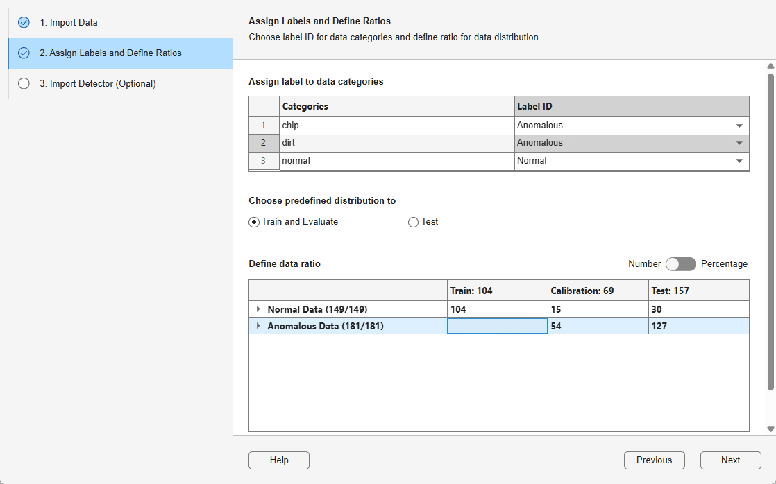
Dialog box with options to assign labels to data categories, choose whether to train and evaluate or to test the data, and define the data ratios using numbers or percentages

You have the option to import a trained detector from the workspace to fine-tune its parameters or evaluate its performance on the imported data. To train a new detector, skip this step and click Done.

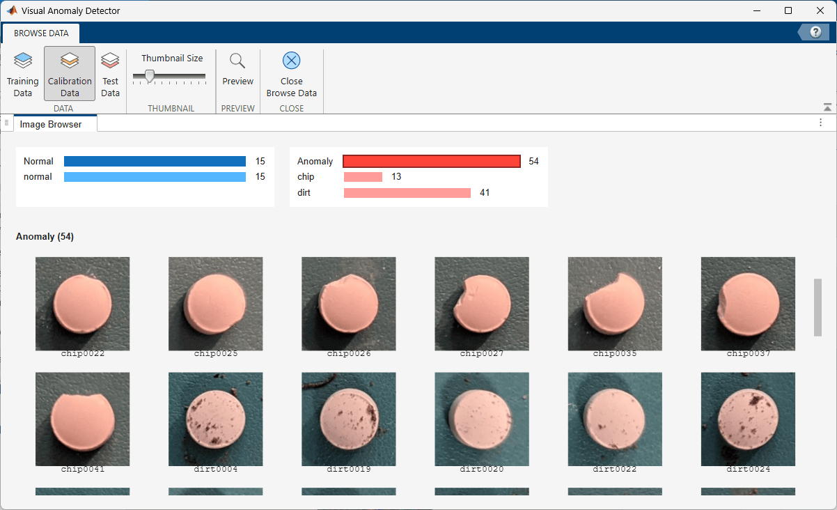
The app opens the Browse Data tab. To view images in each partition, click Training Data, Calibration Data, or Test Data. When you finish reviewing the images, click Close Browse Data to return to the Detector tab. To visualize the imported data again during a session, on the Detector tab, click Visualize.

Browse Data tab with options to view images in the training data, calibration data, or test data

Select and Train Detector

The app selects the StudentTeacher model by default. For this example, train a PatchCore anomaly detector. On the Detector tab of the app toolstrip, select PatchCore from the detectors gallery. The Hyperparameters panel displays the model and training hyperparameters for the selected detector. For more information on these parameters, see patchCoreAnomalyDetector and trainPatchCoreAnomalyDetector. This example uses the default hyperparameters.

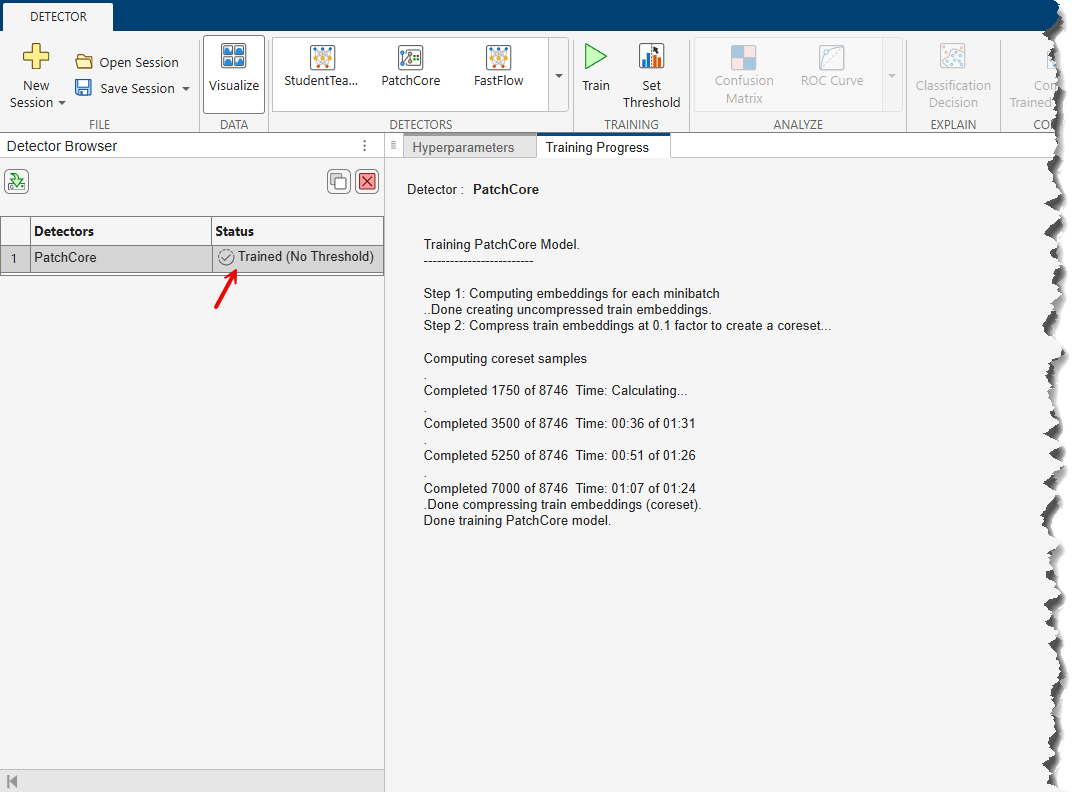
To train the detector, on the Detector tab, click Train. The app starts training the model and displays the progress in the Training Progress panel.

Once training is complete, the app updates the status of the trained detector in the Detector Browser.

Visual Anomaly Detector app with the Detector Browser showing the PatchCore detector status as Trained (No Threshold) and the Training Progress panel showing training details

Set Detection Threshold

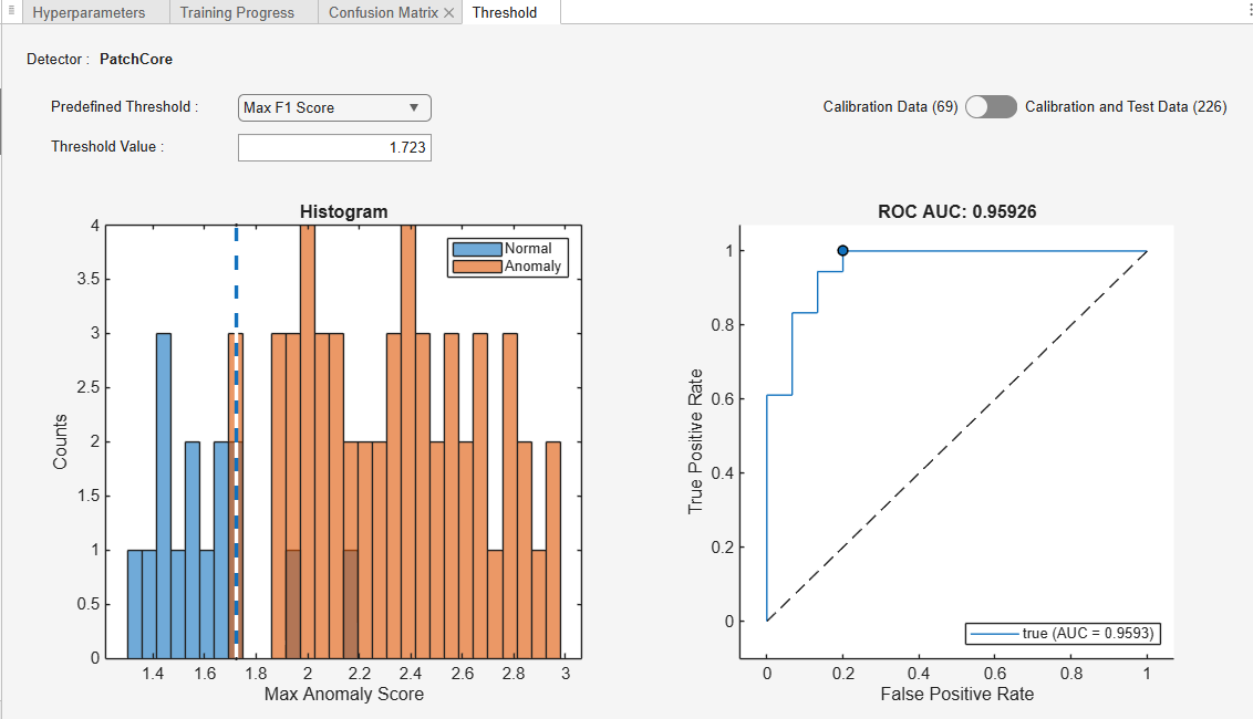
To set the detection threshold, on the Detector tab, click Set Threshold. In the Threshold panel, click the Predefined Threshold list and select one of these options:

Max F1 Score — The threshold that maximizes the balance between precision and recall
Youdens Index — The threshold that maximizes the combined sensitivity and specificity
Nearest Zero-One ROC — The threshold closest to the ideal point on the ROC curve
Custom — A user-defined threshold value

You can also adjust the threshold by entering a new value in Threshold Value box or by interactively dragging the threshold line on the histogram or the operating point on the ROC curve. You can adjust the threshold on only calibration data or both calibration and test data using the toggle switch. For this example, select the Max F1 Score threshold.

Threshold panel showing options to set the threshold value for the PatchCore detector

Visualize and Evaluate Performance

To visualize performance metrics, on the Detector tab of the app toolstrip, select from these options:

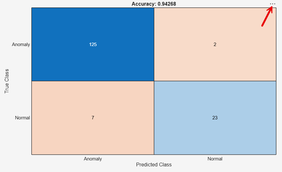
Confusion Matrix — Shows how well the detector performs classification on the test data
ROC Curve — Illustrates the tradeoff between true positive rate and false positive rate across thresholds
Histogram — Displays the distribution of anomaly scores for the normal and anomalous images in the test data
Precision-Recall — Shows how precision and recall change with respect to the threshold
Summary — Summarizes metrics on the test data, including accuracy, sensitivity, and specificity

You can adjust the view and export these plots by clicking the three dots at the top-right corner of the corresponding plots.

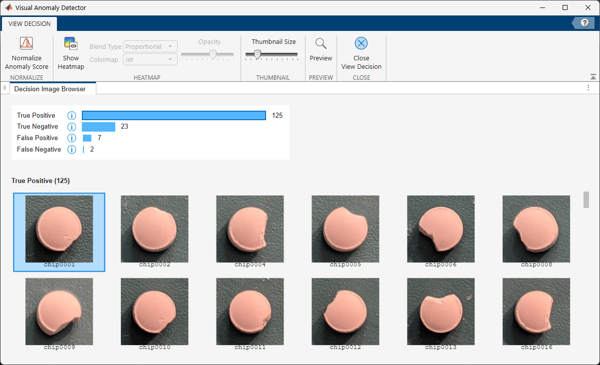
Confusion Matrix visualization for the PatchCore detector. A three-dot button is visible at the top-right corner of the plot.

In addition to these aggregate metrics, you can view classification results on individual images. On the Detector tab, click Classification Decision. The View Decision tab opens and displays test images with their predicted labels. Click the bar of a result category to filter images by that classification.

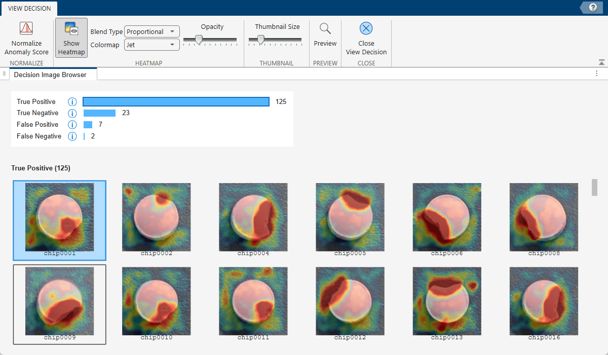
View Decision tab showing result categories of True Positive, True Negative, False Positive, and False Negative, with corresponding images filtered below

In addition to the classification results, you can visualize and evaluate anomaly information using a heatmap overlay to help locate defects. To normalize the anomaly score map using percentile bounds, on the View Decision tab, click Normalize Anomaly Score. In the dialog box that appears, you can accept or adjust the normal image percentile range and the normalized map output range of a normal image. To visualize the anomaly heatmap overlay on images, click Show Heatmap. The heatmap represents the probability of anomaly at each pixel, which helps you understand why the app classified an image as normal or anomalous. Adjust the heatmap visualization using the Blend Type, Colormap, and Opacity controls. To close the visualization, click Close View Decision to return to the Detector tab.

View Decision tab with images that include an anomaly heatmap overlay

Export Trained Model and Performance Data

To export training artifacts, on the Detector tab, click Export, and then select from these options:

Detector — Export the trained detector to the workspace. In the dialog box that opens, specify the variable name. In this example, the detector is saved as a patchCoreAnomalyDetector object.
Training Function — Generate and export a MATLAB function that reproduces the training workflow programmatically. The app creates a .m file and opens it in the MATLAB editor.
Partitioned Datastore — Export the training, calibration, and test datastores to the workspace. In the dialog box that opens, specify the variable names for each ImageDatastore object.
Performance Metrics — Export the evaluation metrics to the workspace. In the dialog box that opens, specify the variable name for the metrics table.

To save the current session for future use, on the Detector tab, select Save Session > Save or Save Session > Save As to save it as a MAT file.

Compare Trained Detectors

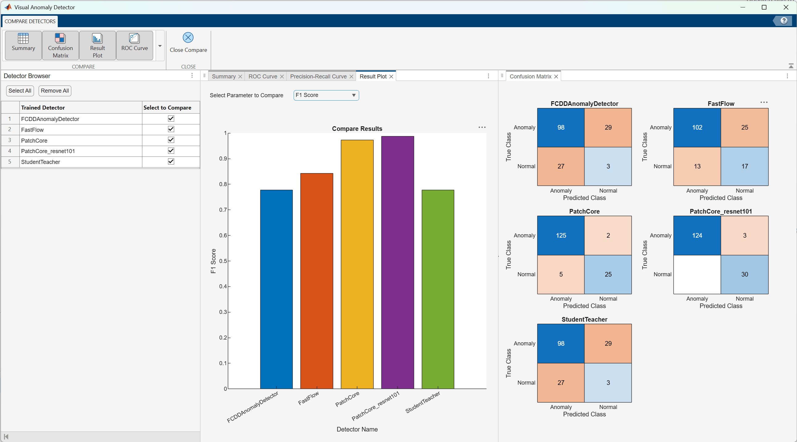
You can train additional detector networks (such as Student-Teacher, FastFlow, or FCDD) in the same app session by selecting additional detectors from the detectors gallery on the Detector tab and following the same training and evaluation steps for each. To compare the performance of multiple trained detectors, on the Detector tab, click Compare Trained Detectors. The Compare Detectors tab opens with a summary table of metrics for all trained detectors. Use the gallery buttons (Summary, ROC Curve, Precision-Recall, Confusion Matrix, and Result Plot) to switch between comparison views.

The specific detection model you select to automate a visual inspection task might depend on several factors. These factors can include the amount of training data available for normal and anomalous samples, the number of anomaly classes to recognize, and the type of localization information required for understanding and monitoring predictions. For more information, see Get Started with Anomaly Detection Using Deep Learning.

Compare Detectors tab showing a F1 Score graphs and confusion matrix for each detector model

References

[1] Taylor, Alex. "PillQC: A pill quality control dataset and associated anomaly detection example." GitHub. January 13, 2022. https://github.com/matlab-deep-learning/pillQC.