Visual Anomaly Detector
R2026bDescription
The Visual Anomaly Detector app enables you to train, fine-tune, evaluate, and compare deep learning-based anomaly detection models for identifying defects in images.
The app supports Student-Teacher, PatchCore, FastFlow, and FCDD (fully convolutional data description) anomaly detector models. For more information on the characteristics and performance of these anomaly detection models, see Get Started with Anomaly Detection Using Deep Learning.
Using this app, you can:
Load and partition labeled image data sets.
Train and fine-tune deep learning anomaly detectors using Student-Teacher, PatchCore, FastFlow, or FCDD architectures.
Evaluate performance with metrics such as confusion matrices, ROC curves, and precision-recall curves.
Optimize detection thresholds using ROC curves and histograms.
Visualize predictions with heatmaps showing anomaly locations.
Compare multiple trained models to select the optimal detector.
Perform inference on production data or live image streams using trained models.
Export models, training functions, partitioned datastores, evaluation metrics and plots.
Open the Visual Anomaly Detector App
MATLAB® Toolstrip: On the Apps tab, under Image Processing and Computer Vision, click the app icon.
MATLAB command prompt: Enter
visualAnomalyDetector. For more information, see Programmatic Use.
Examples
You can open the Visual Anomaly Detector app with pre-partitioned image datastores loaded from the MATLAB workspace.
Create image datastores for training, calibration, and test sets, and specify the anomaly class labels.
imdsTrain = imageDatastore("data/train",IncludeSubfolders=true,LabelSource="foldernames");
imdsCal = imageDatastore("data/calibration",IncludeSubfolders=true,LabelSource="foldernames");
imdsTest = imageDatastore("data/test",IncludeSubfolders=true,LabelSource="foldernames");
anomalyClasses = ["crack","scratch","contamination"];
Open the app with the preloaded data.
visualAnomalyDetector(imdsTrain,imdsCal,imdsTest,anomalyClasses)
The app opens with the data already loaded and partitioned, so you can immediately select a detector and begin training.
Related Examples
Parameters
Use the Detector tab to manage sessions, import training data, select and train anomaly detector models, evaluate performance, and export the trained model, training function, data, or results. The parameters and buttons in this tab are usable only after a session has been created or loaded.
| Parameters/Buttons | Description |
|---|---|
| New Session | Create a new session. Select one of these options from the button menu:
|
| Open Session | Load a previously saved session MAT file. |
| Save Session | Save the current session. Select one of these options from the list:
|
| Visualize | Open the Browse Data tab to browse the imported and partitioned training, calibration, and test data. |
| StudentTeacher | Select the Student-Teacher anomaly detector and display its configurable parameters in the Hyperparameters panel. |
| PatchCore | Select the PatchCore anomaly detector and display its configurable parameters in the Hyperparameters panel. |
| FastFlow | Select the FastFlow anomaly detector and display its configurable parameters in the Hyperparameters panel. |
| FCDD | Select the FCDD (fully convolutional data description) anomaly detector and display its configurable parameters in the Hyperparameters panel. |
| Train | Start training the selected anomaly detector model on the imported training data. Training progress is displayed in the Training Progress panel. Click the button again to stop training. |
| Set Threshold | Open the Threshold panel and configure the anomaly detection threshold. |
| Confusion Matrix | Display the confusion matrix for the test data predictions at the current threshold. |
| ROC Curve | Display the receiver operating characteristic (ROC) curve showing the tradeoff between true positive rate and false positive rate across thresholds. |
| Histogram | Display the histogram of anomaly scores for normal and anomalous images in the test data. |
| Precision-Recall | Display the precision-recall curve for the test data predictions. |
| Summary | Display a summary table of evaluation metrics for the trained detector, including accuracy, precision, recall, and F1 score. |
| Classification Decision | Open the View Decision tab to visualize classification decisions for individual images, including anomaly heatmap overlays. |
| Compare Trained Detectors | Open the Compare Detectors tab to compare the performance of multiple trained detectors side by side. |
| Default Layout | Restore the app window to its default panel layout. |
| Export | Export data to the MATLAB workspace. Select one of these options from the button menu:
|
Use the Browse Data tab to browse and preview the imported and partitioned image datasets. This tab opens when you select Visualize on the Detector tab.
| Parameters/Buttons | Description |
|---|---|
| Training Data | Display thumbnail images from the training data set in the image browser. |
| Calibration Data | Display thumbnail images from the calibration data set in the image browser. |
| Test Data | Display thumbnail images from the test data set in the image browser. |
| Thumbnail Size | Adjust the slider to change the size of thumbnail images displayed in the image browser. |
| Preview | Show or hide a larger preview of the selected image, along with other information, such as assigned label and actual label category. |
| Close Browse Data | Close the Browse Data tab and return to the Detector tab. |
Use the Anomaly Detector: Train / Fine-tune / Evaluate Detector dialog box to import image data and configure a new training session. This dialog box opens when you select New Session > Train / Evaluate on the Detector tab. The dialog box enables you to load data, assign labels, define data distribution, and optionally select pretrained detectors from the workspace.
| Parameters/Buttons | Description |
|---|---|
| Load data from | Select the source of image data. Choose one of these options:
|
| Import ground truth labels | When the selected datastore does not contain labels, you can import ground truth labels separately from the workspace. This option is enabled automatically when labels are not detected in the selected datastore. |
| Assign labels to data categories | Assign each unique label in the imported data to either the
|
| Workflow type | Select the workflow type:
|
| Define data ratio | Specify the data split ratios for partitioning the imported data into training, calibration, and test sets. The tree table displays the distribution per label category. You can edit individual values to customize the allocation. |
| Number/Percent | Choose whether to display the data distribution as absolute image counts or as percentages. |
| Default | Reset the data split ratios to their default values. |
| Select detector to import | Select one or more detectors from the MATLAB workspace to import
into the session. The table includes all trained anomaly detector objects
available in the base workspace. This option is optional for the
|
| Previous | Return to the previous step. |
| Next | Proceed to the next step. This button is enabled only after completing the required selections in the current step. On the final step, the button label changes to Done. |
Use the Anomaly Detector: Perform detection dialog box to import a pretrained anomaly detector model and test data for performing inference. This dialog box opens when you select New Session > Perform Detection.
| Parameters/Buttons | Description |
|---|---|
| Import anomaly detector from workspace | Select trained anomaly detector object from the MATLAB workspace.
The detector must be a |
| Import data from | Select the source folder or datastore containing test images for inference. |
| Import | Load the trained model and test data, and start the inference session. |
Use the Hyperparameters panel to configure model architecture and training hyperparameters for the selected anomaly detector. The available parameters change depending on which detector type you select.
Detector Hyperparameters
| Detector | Parameters | Description |
|---|---|---|
| Student-Teacher | Network | Network size for the Student-Teacher model |
| Normalization Data Ratio | Ratio of training data for anomaly map normalization. Value ranges from 0.0 to 1.0. | |
| PatchCore | Pretrained Backbone Network | Backbone network for feature extraction |
| FastFlow | Pretrained Encoder Network | Encoder network for feature extraction |
| Number of downsampling operations | Number of downsampling layers | |
| FCDD | Pretrained Encoder Network | Encoder network for feature extraction |
| Number of downsampling operations | Number of downsampling layers | |
| Freeze Backbone | Whether to freeze the backbone network weights during training |
For more information on model hyperparameters, see trainStudentTeacherAnomalyDetector, trainPatchCoreAnomalyDetector, trainFastFlowAnomalyDetector, and trainFCDDAnomalyDetector.
Training Hyperparameters
| Parameters | Description |
|---|---|
| Compression Ratio | Ratio for core-set compression. Value ranges from 0.0 to 1.0. |
| Mini-Batch Size | Number of images processed in each mini-batch during feature extraction |
| Execution Environment | Hardware for training |
| Reset Input Normalization | Whether to reset input normalization statistics |
| Subsampling Method | Strategy for subsampling the core set |
| Initial Learn Rate | Initial learning rate for the optimizer |
| Max Epochs | Maximum number of training epochs |
| Stochastic Solver | Optimization algorithm |
| Learn Rate Schedule | Learning rate decay schedule |
| Learn Rate Drop Factor | Factor to reduce the learning rate. Value ranges from 0 to 1. |
| Learn Rate Drop Period | Number of epochs between learning rate drops |
| Shuffle | Data shuffling strategy |
| Momentum | Momentum value for SGDM optimizer |
| Gradient Decay Factor | Decay rate for first moment estimate (beta1) in Adam optimizer |
| Squared Gradient Decay Factor | Decay rate for second moment estimate |
| Epsilon | Small constant for numerical stability |
| Validation Frequency | Number of iterations between validation evaluations |
| Validation Patience | Number of validation checks to wait before stopping early |
| Output Network | Network to return after training |
| L2 Regularization | L2 regularization factor (weight decay) |
| Batch Normalization Statistics | Method for computing batch normalization statistics |
| Gradient Threshold | Threshold for gradient clipping |
| Gradient Threshold Method | Method for gradient clipping |
| Execution Environment | Hardware for training |
| Preprocessing Environment | Data preprocessing parallelization |
| Acceleration | Automatic acceleration for training |
| Checkpoint Path | Folder path to save training checkpoints |
| Checkpoint Frequency | How often to save checkpoints |
| Checkpoint Frequency Unit | Unit for checkpoint frequency |
For more information on these training hyperparameters, see trainingOptions (Deep Learning Toolbox).
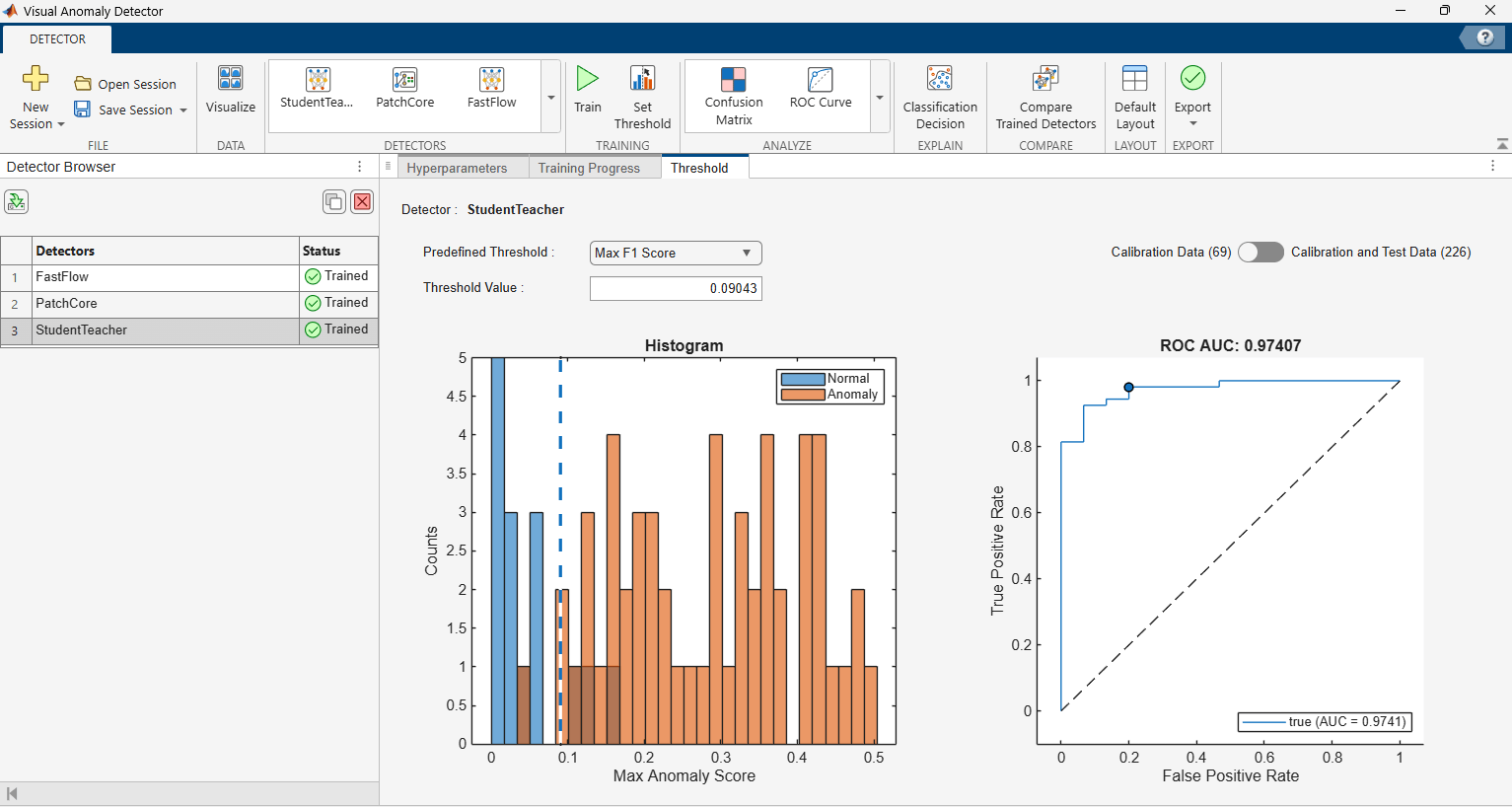
Use the Threshold panel to configure and visualize the anomaly detection threshold. This panel opens when you select Set Threshold on the Detector tab. The threshold determines the decision boundary between normal and anomalous predictions.
| Parameters/Buttons | Description |
|---|---|
| Predefined Threshold | Select one of these threshold method options:
|
| Threshold Value | Numeric threshold value for classification. This value is
automatically set when you select a predefined method. You can enter a
custom value when |
| Data Selection | Select the data for computing the threshold.
|
| ROC Curve | Display ROC curve with the current threshold position indicated on the curve. |
| Histogram | Display the score distribution histogram with the threshold line overlaid, showing separation between normal and anomalous scores. |
You can adjust the view and export these plots, by clicking the three dots at the top-right corner of the corresponding plots.
Use the View Decision tab to visualize classification decisions for individual images, including anomaly heatmap overlays. This tab opens when you select Classification Decision on the Detector tab.
| Parameters/Buttons | Description |
|---|---|
| Normalize Anomaly Score | Open a dialog box for configuring anomaly score normalization settings. |
| Show Heatmap | Toggle the visibility of the anomaly heatmap overlay on images. |
| Blend Type | Select a blending method for the heatmap overlay. Use
|
| Colormap | Select the colormap for the anomaly heatmap. |
| Opacity | Adjust the opacity of the heatmap overlay. Range is 1 to 100. |
| Thumbnail Size | Adjust the size of image thumbnails in the decision browser. |
| Preview | Show or hide a larger preview of the selected image with heatmap overlay. |
| Close View Decision | Close the View Decision tab and return to the Detector tab. |
Use the Compare Detectors tab to compare the performance of multiple trained anomaly detectors side by side. This tab opens when you select Compare Trained Detectors on the Detector tab.
| Parameters/Buttons | Description |
|---|---|
| Model Selection | Select which models to include in the comparison from the left panel which lists all trained detectors. Use Select All to include all detectors or Remove All to clear the selection. The comparison views update dynamically as you change the selection. |
| Summary | Display a comparison summary table of evaluation metrics for the selected detectors. The table shows metrics such as Global Accuracy, Mean Accuracy, Precision, Recall, Specificity, F1 Score, False Positive Rate, False Negative Rate, and Model Type. Click Select Parameter to customize which metrics appear as columns in the table. Click Export to Workspace to export the summary table to the MATLAB workspace as a table. |
| Result Plot | Display a bar chart comparing a selected metric across all selected detectors. Use the Select parameter to compare list to choose the metric to plot. Available metrics include Global Accuracy, Mean Accuracy, Precision, Recall, Specificity, F1 Score, False Positive Rate, and False Negative Rate. |
| ROC Curve | Display overlaid ROC curves for all selected detectors on a single plot, enabling direct comparison of the tradeoff between true positive rate and false positive rate across detectors. |
| Confusion Matrix | Display confusion matrices for all selected detectors in a tiled layout for side-by-side comparison of classification results. |
| Precision-Recall | Display overlaid precision-recall curves for all selected detectors on a single plot, enabling direct comparison of the tradeoff between precision and recall across detectors. |
| Close Compare | Close the Compare Detectors tab and return to the Detector tab. |
Use the Connect Device dialog box to connect to an image acquisition device for live anomaly detection. This dialog box opens when you select New Session > Live Detection. This feature requires Image Acquisition Toolbox.
| Parameters/Buttons | Description |
|---|---|
| Select Device | Select an image acquisition device (camera) for capturing live images. Use the refresh button to refresh the list of available devices. |
| Select Pixel Format | Select the pixel format of the image stream. |
| Connect | Establish a connection to the selected device and begin the live detection session. |
Use the Live Detection tab to perform real-time anomaly detection on live image streams captured from a connected image acquisition device. This tab opens when you select New Session > Live Detection and connect a device using the Connect Device dialog box. This feature requires Image Acquisition Toolbox.
| Parameters/Buttons | Description |
|---|---|
| Detector | Select a trained anomaly detector from the MATLAB workspace. The list includes all anomaly detector objects available in the base workspace. Use the refresh button to refresh the list of available anomaly detectors from the MATLAB workspace. |
| Start | Begin capturing images from the connected device and running the selected anomaly detector on each captured frame in real time. The button changes to Stop while detection is active. |
| Heat Map | Toggle the anomaly heatmap overlay on the live image stream.
Options are |
| Opacity | Adjust the opacity of the heatmap overlay on the live image. Range
is 1 to 100. Default is |
| Switch Device | Adjust the device properties such as the connected device and pixel format. |
| Device Properties | Adjust the properties of the connected device, such as the ROI, frame rate, and saturation. |
| Live Image Display | View the live image stream from the connected device with real-time classification annotations. The app annotates each frame with the detection result (Good or Bad) and the anomaly score. |
Programmatic Use
visualAnomalyDetector opens the Visual Anomaly Detector
app.
visualAnomalyDetector(imdsTrain,imdsCal,imdsTest,anomalyClasses)
opens the Visual Anomaly Detector app with pre-partitioned image data loaded from
the workspace.
imdsTrain— Image datastore containing training images, specified as anImageDatastoreobject.imdsCal— Image datastore containing calibration images used for threshold optimization, specified as anImageDatastoreobject.imdsTest— Image datastore containing test images for evaluating detector performance, specified as anImageDatastoreobject.anomalyClasses— Names of the classes that represent anomalous images, specified as a string array or categorical array. The app treats all other class labels in the datastores as normal.
visualAnomalyDetector close closes the Visual Anomaly
Detector app.
Version History
Introduced in R2026b
See Also
Functions
MATLAB Command
You clicked a link that corresponds to this MATLAB command:
Run the command by entering it in the MATLAB Command Window. Web browsers do not support MATLAB commands.


选择网站
选择网站以获取翻译的可用内容,以及查看当地活动和优惠。根据您的位置,我们建议您选择:。
您也可以从以下列表中选择网站:
如何获得最佳网站性能
选择中国网站(中文或英文)以获得最佳网站性能。其他 MathWorks 国家/地区网站并未针对您所在位置的访问进行优化。
美洲
- América Latina (Español)
- Canada (English)
- United States (English)
欧洲
- Belgium (English)
- Denmark (English)
- Deutschland (Deutsch)
- España (Español)
- Finland (English)
- France (Français)
- Ireland (English)
- Italia (Italiano)
- Luxembourg (English)
- Netherlands (English)
- Norway (English)
- Österreich (Deutsch)
- Portugal (English)
- Sweden (English)
- Switzerland
- United Kingdom (English)