csymwavf
Syntax
Description
f = csymwavf(wname)wname.
To learn which functions support complex symlets, see Discrete Wavelet Transform Functions and Complex Symlets.
Examples
Obtain the scaling filter associated with the complex symlet with four vanishing moments.
n = 4;
scf = csymwavf("csym"+num2str(n));
Confirm that the filter coefficients are normalized such that their sum is equal to 1.
sum(scf)
ans =
1.0000 + 0.0000i
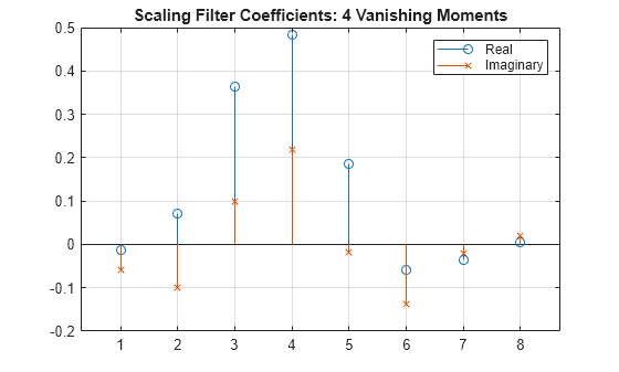
Plot the real and imaginary parts of the filter coefficients. Because the symlet has an even number of vanishing moments, the filter coefficients are not symmetric about the midpoint.
stem(real(scf),"o-")
hold on
stem(imag(scf),"x-")
hold off
grid on
legend("Real","Imaginary")
title("Scaling Filter Coefficients: "+num2str(n)+" Vanishing Moments")
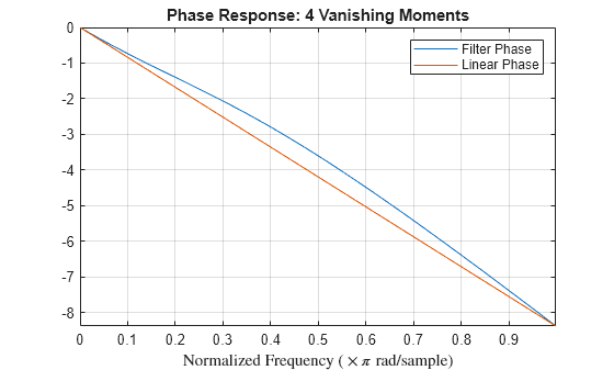
Use the function phasez (Signal Processing Toolbox) to plot the phase response. Because the complex symlet is an orthogonal wavelet with compact support, the filter response deviates noticeably from linear phase.
[phz,w] = phasez(scf);

plot(w/pi,phz)
hold on
plot([w(1)/pi w(end)/pi], [phz(1) phz(end)])
grid on
hold off
axis tight
legend("Filter Phase","Linear Phase")
title("Phase Response: "+num2str(n)+" Vanishing Moments")
xlabel("Normalized Frequency ($\times\pi$ rad/sample)", ...
    "Interpreter","latex")
Obtain the scaling filter associated with the complex symlet with five vanishing moments.
n = 5;
scf = csymwavf("csym"+num2str(n));
Confirm the filter coefficients are normalized such that their sum is equal to 1.
sum(scf)
ans =
1.0000 - 0.0000i
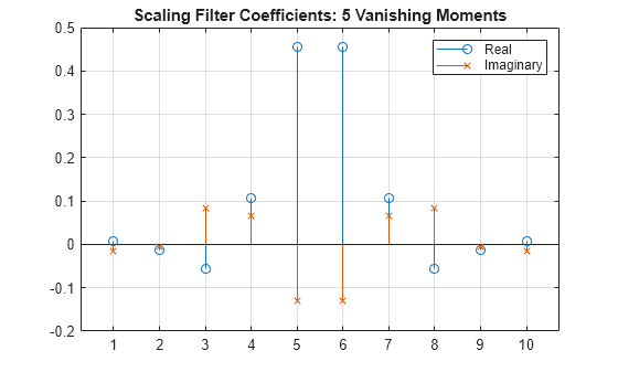
Plot the real and imaginary parts of the filter coefficients. Because the symlet has an odd number of vanishing moments, the filter coefficients are symmetric about the midpoint.
stem(real(scf),"o-")
hold on
stem(imag(scf),"x-")
hold off
grid on
legend("Real","Imaginary")
title("Scaling Filter Coefficients: "+num2str(n)+" Vanishing Moments")
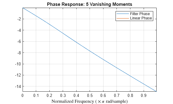
Plot the phase response. With an odd number of vanishing moments, you can get almost linear phase.
[phz,w] = phasez(scf);

plot(w/pi,phz)
hold on
plot([w(1)/pi w(end)/pi], [phz(1) phz(end)])
grid on
hold off
axis tight
legend("Filter Phase","Linear Phase")
title("Phase Response: "+num2str(n)+" Vanishing Moments")
xlabel("Normalized Frequency ($\times\pi$ rad/sample)", ...
    "Interpreter","latex")
Input Arguments
Output Arguments
More About
References
[1] Daubechies, Ingrid. “Orthonormal Bases of Compactly Supported Wavelets.” Communications on Pure and Applied Mathematics 41, no. 7 (1988): 909–96. https://doi.org/10.1002/cpa.3160410705.
[2] Lawton, W. “Applications of Complex Valued Wavelet Transforms to Subband Decomposition.” IEEE Transactions on Signal Processing 41, no. 12 (1993): 3566–68. https://doi.org/10.1109/78.258098.
[3] Lina, Jean-Marc, and Michel Mayrand. “Complex Daubechies Wavelets.” Applied and Computational Harmonic Analysis 2, no. 3 (1995): 219–29. https://doi.org/10.1006/acha.1995.1015.
[4] Xiao-Ping Zhang, M.D. Desai, and Ying-Ning Peng. “Orthogonal Complex Filter Banks and Wavelets: Some Properties and Design.” IEEE Transactions on Signal Processing 47, no. 4 (1999): 1039–48. https://doi.org/10.1109/78.752601.
Extended Capabilities
Version History
Introduced in R2026a