daubfactors

Daubechies wavelet families scaling filter computation

Since R2026a

Syntax

h = daubfactors(n,fsn)

Description

h = daubfactors(n,fsn) returns the scaling (lowpass reconstruction) filter with n vanishing moments for the Daubechies wavelet family specified by fsn.

example

Examples

collapse all

Quadrature Mirror Filters for Daubechies Wavelet Families

Open Live Script

Use the function daubfactors to obtain the quadrature mirror filters associated with a member of each Daubechies wavelet family.

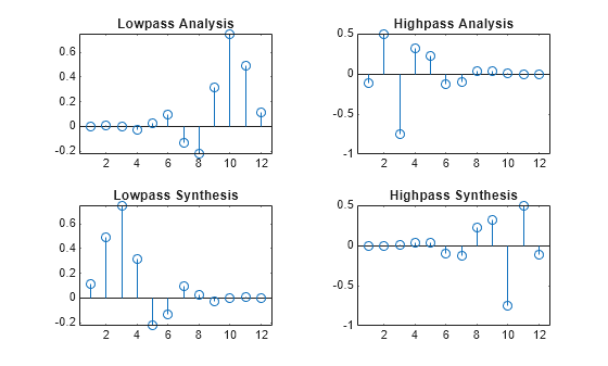
Extremal Phase Wavelet

Obtain the scaling filter associated with the extremal phase wavelet with 6 vanishing moments. Confirm that the sum of the filter coefficients is 1.

n = 6;
wvf = "db";
h = daubfactors(n,wvf);
sum(h)

ans = 
1

Use the function orthfilt to obtain the quadrature mirror filters associated with the wavelet. The first filter pair lod and hid are the lowpass and highpass decomposition (analysis) filters, respectively. The second filter pair lor and hir are the lowpass and highpass reconstruction (synthesis) filters, respectively. Plot the filters.

[lod,hid,lor,hir] = orthfilt(h);

tiledlayout(2,2)
nexttile
stem(lod)
title("Lowpass Analysis")
nexttile
stem(hid)
title("Highpass Analysis")
nexttile
stem(lor)
title("Lowpass Synthesis")
nexttile
stem(hir)
title("Highpass Synthesis")

Figure contains 4 axes objects. Axes object 1 with title Lowpass Analysis contains an object of type stem. Axes object 2 with title Highpass Analysis contains an object of type stem. Axes object 3 with title Lowpass Synthesis contains an object of type stem. Axes object 4 with title Highpass Synthesis contains an object of type stem.

Choose a filter pair and use the function isorthwfb to confirm that the filter bank satisfies the necessary and sufficient conditions to be a two-channel orthonormal perfect reconstruction filter bank.

[tf,checks] = isorthwfb(lod,hid) %#ok<*ASGLU>

tf = logical
   1

checks=7×3 table
                                          Pass-Fail    Maximum Error    Test Tolerance
                                          _________    _____________    ______________

    Equal-length filters                    pass                 0                 0  
    Even-length filters                     pass                 0                 0  
    Unit-norm filters                       pass        2.2204e-16        1.4901e-08  
    Filter sums                             pass        1.2186e-16        1.4901e-08  
    Even and odd downsampled sums           pass        1.1102e-16        1.4901e-08  
    Zero autocorrelation at even lags       pass        6.5285e-16        1.4901e-08  
    Zero crosscorrelation at even lags      pass        2.7756e-17        1.4901e-08

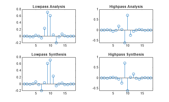
Least Asymmetric Wavelet

Obtain the scaling filter associated with the least asymmetric wavelet with 5 vanishing moments. Confirm that the sum of the filter coefficients is 1.

n = 9;
wvf = "sym";
h = daubfactors(n,wvf);
sum(h)

ans = 
1.0000

Obtain the associated quadrature mirror filters.

[lod,hid,lor,hir] = orthfilt(h);

tiledlayout(2,2)
nexttile
stem(lod)
title("Lowpass Analysis")
nexttile
stem(hid)
title("Highpass Analysis")
nexttile
stem(lor)
title("Lowpass Synthesis")
nexttile
stem(hir)
title("Highpass Synthesis")

Use the scaling filter that daubfactors returns to confirm that the filter bank formed from the filter defines a two-channel orthonormal perfect reconstruction filter bank.

[tf,checks] = isorthwfb(h)

tf = logical
   1

checks=7×3 table
                                          Pass-Fail    Maximum Error    Test Tolerance
                                          _________    _____________    ______________

    Equal-length filters                    pass                 0                 0  
    Even-length filters                     pass                 0                 0  
    Unit-norm filters                       pass        2.4425e-15        1.4901e-08  
    Filter sums                             pass        8.8818e-16        1.4901e-08  
    Even and odd downsampled sums           pass        2.2204e-16        1.4901e-08  
    Zero autocorrelation at even lags       pass         1.145e-15        1.4901e-08  
    Zero crosscorrelation at even lags      pass        2.1491e-17        1.4901e-08

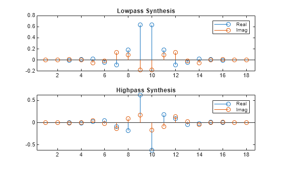
Complex Symlet

Obtain the scaling filter associated with the complex symlet with 11 vanishing moments. Confirm that the sum of the filter coefficients is 1.

n = 9;
wvf = "csym";
h = daubfactors(n,wvf);
sum(h)

ans = 
1.0000 + 0.0000i

Obtain the associated quadrature mirror filters. Plot the real and imaginary parts of the synthesis filters. Because the complex symlet has an odd number of vanishing moments, the lowpass filter is symmetric about the midpoint.

[lod,hid,lor,hir] = orthfilt(h);

tiledlayout(2,1)
nexttile
stem([real(lor).'  imag(lor).'])
title("Lowpass Synthesis")
legend("Real","Imag")
nexttile
stem([real(hir).'  imag(hir).'])
title("Highpass Synthesis")
legend("Real","Imag")

Figure contains 2 axes objects. Axes object 1 with title Lowpass Synthesis contains 2 objects of type stem. These objects represent Real, Imag. Axes object 2 with title Highpass Synthesis contains 2 objects of type stem. These objects represent Real, Imag.

Confirm that the filter bank defines a two-channel orthonormal perfect reconstruction filter bank.

[tf,checks] = isorthwfb(lor,hir)

tf = logical
   1

checks=7×3 table
                                          Pass-Fail    Maximum Error    Test Tolerance
                                          _________    _____________    ______________

    Equal-length filters                    pass                 0                 0  
    Even-length filters                     pass                 0                 0  
    Unit-norm filters                       pass        2.1094e-15        1.4901e-08  
    Filter sums                             pass        2.2508e-16        1.4901e-08  
    Even and odd downsampled sums           pass        2.2214e-16        1.4901e-08  
    Zero autocorrelation at even lags       pass        2.9177e-15        1.4901e-08  
    Zero crosscorrelation at even lags      pass        2.4252e-17        1.4901e-08

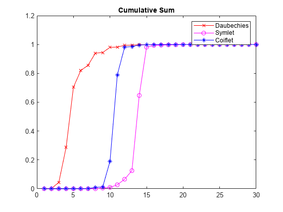
Demonstrate Extremal Phase Property

Open Live Script

For a given support, the cumulative sum of the squared coefficients of a scaling filter increases more rapidly for an extremal phase wavelet than other wavelets.

Generate the scaling filter coefficients for the db15 and sym15 wavelets. Both wavelets have support of width $2 \times 15 - 1 = 29$ .

n = 15;
lor_db = daubfactors(n);
lor_sym = daubfactors(n,"sym");

Next, generate the scaling filter coefficients for the coif5 wavelet. This wavelet also has support of width $6 \times 5 - 1 = 29$ .

lor_coif = coifwavf("coif5");

Confirm that the sum of the coefficients for all three wavelets equals 1.

sum(lor_db)

ans = 
1.0000

sum(lor_sym)

ans = 
1.0000

sum(lor_coif)

ans = 
1.0000

Plot the cumulative sums of the squared coefficients. Note how rapidly the Daubechies sum increases. The sum increases rapidly because its energy is concentrated at small abscissas. Since the Daubechies wavelet has extremal phase, the cumulative sum of its squared coefficients increases more rapidly than the other two wavelets.

plot(cumsum(lor_db.^2),"x-")
hold on
plot(cumsum(lor_sym.^2),"o-")
plot(cumsum(lor_coif.^2),"*-")
hold off
legend("Daubechies","Symlet","Coiflet")
title("Cumulative Sum")

Figure contains an axes object. The axes object with title Cumulative Sum contains 3 objects of type line. These objects represent Daubechies, Symlet, Coiflet.

Least Asymmetric Wavelet and Phase

This example uses:

Open Live Script

Obtain the scaling filter associated with the symlet of order 4.

n = 4;
scal_sym = daubfactors(n,"sym");

Use the function freqz (Signal Processing Toolbox) to plot the frequency response of the filter. Compare the phase angle with a linear phase filter.

freqz(scal_sym)
subPlots = get(gcf,"Children");
phasePlot = subPlots(2);
yLimits = get(phasePlot,"Ylim");
hold(phasePlot,"on");
plot(phasePlot,[0 1],[0 yLimits(1)])
legend(phasePlot,"Symlet","Linear")
hold(phasePlot,"off")

$Figure contains 2 axes objects. Axes object 1 with title Phase, xlabel Normalized Frequency (\times\pi rad/sample), ylabel Phase (degrees) contains 2 objects of type line. These objects represent Symlet, Linear. Axes object 2 with title Magnitude, xlabel Normalized Frequency (\times\pi rad/sample), ylabel Magnitude (dB) contains an object of type line.$

Obtain the scaling filter associated with the Daubechies wavelet of order 4. Plot the frequency response of the filter. Compare the phase angle with a linear phase filter.

db_sym = daubfactors(n);

freqz(db_sym)
subPlots = get(gcf,"Children");
phasePlot = subPlots(2);
yLimits = get(phasePlot,"Ylim");
hold(phasePlot,"on");
plot(phasePlot,[0 1],[0 yLimits(1)])
legend(phasePlot,"Daubechies","Linear")
hold(phasePlot,"off")

$Figure contains 2 axes objects. Axes object 1 with title Phase, xlabel Normalized Frequency (\times\pi rad/sample), ylabel Phase (degrees) contains 2 objects of type line. These objects represent Daubechies, Linear. Axes object 2 with title Magnitude, xlabel Normalized Frequency (\times\pi rad/sample), ylabel Magnitude (dB) contains an object of type line.$

Input Arguments

collapse all

`n` — Number of vanishing moments
positive integer

Number of vanishing moments of the lowpass filter, specified as a positive integer less than or equal to 45. The minimum number of vanishing moments you can specify depends on the Daubechies wavelet family:

Extremal phase ("db") and least asymmetric ("sym") — Minimum number is 1
Complex symlet ("csym") — Minimum number is 3

For n equal to 1, 2 and 3, the order n extremal phase and least asymmetric wavelets are identical.

Note

You might encounter numerical instability when n is too large. Beginning with values of n in the range [30,40], the vector output of daubfactors no longer accurately represents scaling filter coefficients.

Data Types: double

`fsn` — Daubechies wavelet family short name
`"db"` (default) | `"sym"` | `"csym"`

Daubechies wavelet family short name, specified as one of these:

"db" — Daubechies extremal phase wavelet. For more information, Extremal Phase Wavelet.
"sym" — Daubechies least asymmetric wavelet. For more information, see Least Asymmetric Wavelet.
"csym" — Complex symlet (complex-valued least asymmetric Daubechies wavelet). For more information, see Complex Symlets.

Output Arguments

collapse all

`h` — Scaling filter
vector

Scaling filter, returned as a vector. The function normalizes the filter such that the sum of the filter coefficients equals 1.

More About

collapse all

Extremal Phase Wavelet

An extremal phase wavelet is a compactly supported orthogonal wavelet whose associated scaling filter is such that all the zeros of the filter are inside the unit circle in the complex plane. For a given support width, extremal phase wavelets have the highest number of vanishing moments.

Constructing a compactly supported orthogonal wavelet basis involves choosing roots of a particular polynomial equation. Different choices of roots result in wavelets whose phases are different. Choosing roots that lie within the unit circle in the complex plane results in a filter with highly nonlinear phase. Such a wavelet is said to have extremal phase, and has energy concentrated at small abscissas. Let {h_k} denote the set of scaling coefficients associated with an extremal phase wavelet, where k = 1,…,M. Then for any other set of scaling coefficients {g_k} resulting from a different choice of roots, the following inequality holds for all J = 1,…,M:

$\sum_{k = 1}^{J} g_{k}^{2} \leq \sum_{k = 1}^{J} h_{k}^{2} .$

The {h_k} are sometimes called a minimal delay filter.

The polynomial equation depends on the number of vanishing moments N for the wavelet. To construct a wavelet basis involves choosing roots of the equation. In the case of least asymmetric wavelets and extremal phase wavelets of orders 1, 2, and 3, there are effectively no choices to make. For N = 1, 2, and 3, the dbN and symN filters are equal.

Least Asymmetric Wavelet

For a given support width, a least asymmetric wavelet is an orthogonal wavelet with phase response that most closely resembles a linear phase filter.

The Haar wavelet, also known as the Daubechies wavelet of order 1, db1, is the only compactly supported orthogonal wavelet that is symmetric, or equivalently has linear phase. No other compactly supported orthogonal wavelet can be symmetric.

Complex Symlets

Complex symlets are complex-valued least asymmetric Daubechies wavelets. Complex symlets have the highest number of vanishing moments for a given support width. The associated scaling filters have near-linear phase response and are symmetric for odd numbers of vanishing moments and least asymmetric for even numbers of vanishing moments. The minimum number of vanishing moments a complex symlet can have is 3.

In [3], Daubechies showed that the db1 (Haar) wavelet is the only compactly supported real-valued orthogonal wavelet that is symmetric, or equivalently, has linear phase. For a given support, a symlet is a least asymmetric orthogonal wavelet. Its phase response most closely resembles a linear phase filter. Lawton [4] and Lina and Maynard [5] discovered that symmetric complex-valued orthogonal wavelets with compact support, also known as complex-valued Daubechies wavelets, exist. These wavelets do not have linear phase. Zhang, Desai, and Peng [6] proposed a method for constructing complex symlets, complex-valued least asymmetric Daubechies wavelet filters with approximately linear phase.

To learn which functions support complex symlets, see Discrete Wavelet Transform Functions and Complex Symlets.

References

[1] Shensa, M.J. “The Discrete Wavelet Transform: Wedding the a Trous and Mallat Algorithms.” IEEE Transactions on Signal Processing 40, no. 10 (1992): 2464–82. https://doi.org/10.1109/78.157290.

[2] Daubechies, I. Ten Lectures on Wavelets, CBMS-NSF Regional Conference Series in Applied Mathematics. Philadelphia, PA: SIAM Ed, 1992.

[3] Daubechies, Ingrid. “Orthonormal Bases of Compactly Supported Wavelets.” Communications on Pure and Applied Mathematics 41, no. 7 (1988): 909–96. https://doi.org/10.1002/cpa.3160410705.

[4] Lawton, W. “Applications of Complex Valued Wavelet Transforms to Subband Decomposition.” IEEE Transactions on Signal Processing 41, no. 12 (1993): 3566–68. https://doi.org/10.1109/78.258098.

[5] Lina, Jean-Marc, and Michel Mayrand. “Complex Daubechies Wavelets.” Applied and Computational Harmonic Analysis 2, no. 3 (1995): 219–29. https://doi.org/10.1006/acha.1995.1015.

[6] Xiao-Ping Zhang, M.D. Desai, and Ying-Ning Peng. “Orthogonal Complex Filter Banks and Wavelets: Some Properties and Design.” IEEE Transactions on Signal Processing 47, no. 4 (1999): 1039–48. https://doi.org/10.1109/78.752601.

Extended Capabilities

expand all

C/C++ Code Generation
Generate C and C++ code using MATLAB® Coder™.

GPU Code Generation
Generate CUDA® code for NVIDIA® GPUs using GPU Coder™.

GPU Arrays
Accelerate code by running on a graphics processing unit (GPU) using Parallel Computing Toolbox™.

The daubfactors function fully supports GPU arrays. To run the function on a GPU, specify the input data as a gpuArray (Parallel Computing Toolbox). For more information, see Run MATLAB Functions on a GPU (Parallel Computing Toolbox).

Version History

Introduced in R2026a

daubfactors

Syntax

Description

Examples

Quadrature Mirror Filters for Daubechies Wavelet Families

Demonstrate Extremal Phase Property

Least Asymmetric Wavelet and Phase

Input Arguments

`n` — Number of vanishing moments
positive integer

`fsn` — Daubechies wavelet family short name
`"db"` (default) | `"sym"` | `"csym"`

Output Arguments

`h` — Scaling filter
vector

More About

Extremal Phase Wavelet

Least Asymmetric Wavelet

Complex Symlets

References

Extended Capabilities

C/C++ Code Generation
Generate C and C++ code using MATLAB® Coder™.

GPU Code Generation
Generate CUDA® code for NVIDIA® GPUs using GPU Coder™.

GPU Arrays
Accelerate code by running on a graphics processing unit (GPU) using Parallel Computing Toolbox™.

Version History

See Also

Topics

daubfactors

Syntax

Description

Examples

Quadrature Mirror Filters for Daubechies Wavelet Families

Demonstrate Extremal Phase Property

Least Asymmetric Wavelet and Phase

Input Arguments

n — Number of vanishing moments positive integer

fsn — Daubechies wavelet family short name "db" (default) | "sym" | "csym"

Output Arguments

h — Scaling filter vector

More About

Extremal Phase Wavelet

Least Asymmetric Wavelet

Complex Symlets

References

Extended Capabilities

C/C++ Code Generation Generate C and C++ code using MATLAB® Coder™.

GPU Code Generation Generate CUDA® code for NVIDIA® GPUs using GPU Coder™.

GPU Arrays Accelerate code by running on a graphics processing unit (GPU) using Parallel Computing Toolbox™.

Version History

See Also

Topics

`n` — Number of vanishing moments
positive integer

`fsn` — Daubechies wavelet family short name
`"db"` (default) | `"sym"` | `"csym"`

`h` — Scaling filter
vector

C/C++ Code Generation
Generate C and C++ code using MATLAB® Coder™.

GPU Code Generation
Generate CUDA® code for NVIDIA® GPUs using GPU Coder™.

GPU Arrays
Accelerate code by running on a graphics processing unit (GPU) using Parallel Computing Toolbox™.