Main Content

orthfilt

Orthogonal wavelet filters

Description

[LoD,HiD,LoR,HiR] = orthfilt(W) computes the four lowpass and highpass, decomposition and reconstruction filters associated with the scaling filter W corresponding to a wavelet.

example

Examples

collapse all

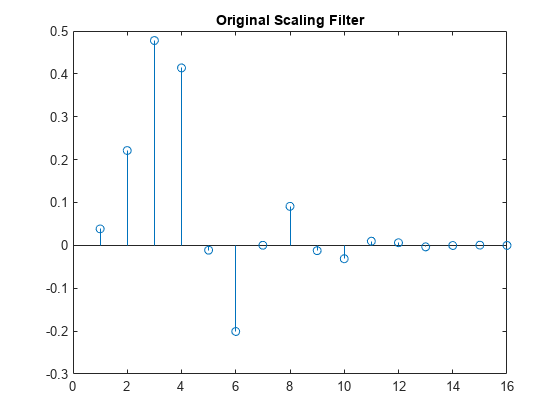
Create a scaling filter associated with the Daubechies db8 wavelet.

W = dbwavf("db8"); 
stem(W)
title("Original Scaling Filter")

Figure contains an axes object. The axes object with title Original Scaling Filter contains an object of type stem.

Compute the four filters associated with the scaling filter.

[LoD,HiD,LoR,HiR] = orthfilt(W); 

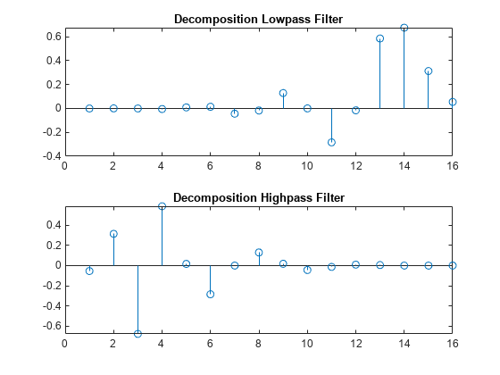
Plot the decomposition lowpass and highpass filters.

subplot(2,1,1)
stem(LoD)
title("Decomposition Lowpass Filter")
subplot(2,1,2)
stem(HiD)
title("Decomposition Highpass Filter")

Figure contains 2 axes objects. Axes object 1 with title Decomposition Lowpass Filter contains an object of type stem. Axes object 2 with title Decomposition Highpass Filter contains an object of type stem.

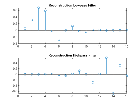
Plot the reconstruction lowpass and highpass filters.

subplot(2,1,1)
stem(LoR)
title("Reconstruction Lowpass Filter")
subplot(2,1,2)
stem(HiR)
title("Reconstruction Highpass Filter")

Figure contains 2 axes objects. Axes object 1 with title Reconstruction Lowpass Filter contains an object of type stem. Axes object 2 with title Reconstruction Highpass Filter contains an object of type stem.

Check for orthonormality in the decomposition filters.

df = [LoD;HiD];
rf = [LoR;HiR];
id = df*df'
id = 2×2

    1.0000   -0.0000
   -0.0000    1.0000

Check for orthonormality in the reconstruction filters.

id2 = rf*rf'
id2 = 2×2

    1.0000    0.0000
    0.0000    1.0000

Check for orthogonality by dyadic translation.

df = [LoD 0 0;HiD 0 0]; 
dft = [0 0 LoD; 0 0 HiD]; 
zer = df*dft'
zer = 2×2
10-12 ×

   -0.1895   -0.0000
    0.0000   -0.1895

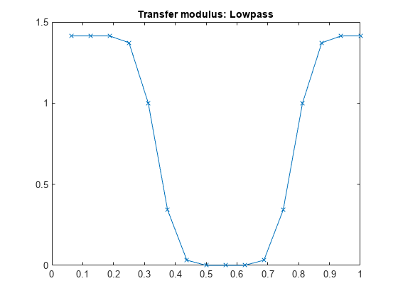
Plot the low-frequency transfer modulus.

fftld = fft(LoD); 
freq = [1:length(LoD)]/length(LoD); 
figure
plot(freq,abs(fftld),"x-")
title("Transfer modulus: Lowpass")

Figure contains an axes object. The axes object with title Transfer modulus: Lowpass contains an object of type line.

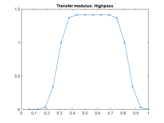
Plot the high-frequency transfer modulus.

ffthd = fft(HiD);
plot(freq,abs(ffthd),"x-")
title("Transfer modulus: Highpass")

Figure contains an axes object. The axes object with title Transfer modulus: Highpass contains an object of type line.

Input Arguments

collapse all

Scaling filter corresponding to a wavelet, specified as a real-valued vector.

Output Arguments

collapse all

Decomposition lowpass filter associated with the scaling filter W, returned as a real-valued vector.

Decomposition highpass filter associated with the scaling filter W, returned as a real-valued vector.

Reconstruction lowpass filter associated with the scaling filter W, returned as a real-valued vector.

Reconstruction highpass filter associated with the scaling filter W, returned as a real-valued vector.

Algorithms

For an orthogonal wavelet in the multiresolution framework, start with the scaling function ϕ and the wavelet function ψ. One of the fundamental relations is the twin-scale relation:

12ϕ(x2)=nZwnϕ(xn)

All the filters used in the dwt and idwt functions are intimately related to the sequence (wn)nZ. If ϕ is compactly supported, the sequence (wn) is finite and can be viewed as an FIR filter. The scaling filter W is a lowpass FIR filter of length 2N, with the sum 1, and with the norm of 1/√2.

For example, for a db3 scaling filter,

w = dbwavf("db3") 
w = 0.2352 0.5706 0.3252 -0.0955 -0.0604 0.0249

sum(w)
 = 1.000
norm(w)
 = 0.7071

Define four FIR filters from filter W of length 2N and norm 1.

Filters

Low-Pass

High-Pass

Decomposition

LoDHiD

Reconstruction

LoRHiR

The function computes the four filters using the following scheme.
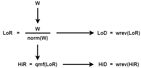
HiR and LoR are quadrature mirror filters: HiR(k) = (-1)kLoR(2N + 1 - k), for k = 1, 2, … , 2N. Because wrev reverses vectors, HiD and LoD are also quadrature mirror filters.

References

[1] Daubechies, Ingrid. Ten Lectures on Wavelets. CBMS-NSF Regional Conference Series in Applied Mathematics 61. Philadelphia, Pa: Society for Industrial and Applied Mathematics, 1992.
Extended Capabilities

C/C++ Code Generation
Generate C and C++ code using MATLAB® Coder™.

Version History

Introduced before R2006a

See Also

| |